 |
| |||||
|
| ||||||||
|
| ||||||||
Home  Publications Publications |
|
|
Note to the Reader This is a revised version of a paper published in The Journal of Comparative in 1986. Several figures have been added. Additions are delimited by brackets [...]. Enlarging images: Thumbnail versions of all figures are embedded in the paper. A better image—usually under 100K—will download into a separate window if you click on the thumbnail image. If you have a large enough monitor drag this second figures window beside the text window. Finally, high-resolution images—usually under 600K—that almost match the quality of the original prints can be downloaded by selecting the text at the bottom of each legend. These image files can be viewed with Adobe Photoshop, NIH Image, or equivalent. Revised HTML edition (http://www.nervenet.org/papers/cat86.html) copyright © 1998 by Robert W. Williams.
PDF version The Journal of Comparative Neurology 246:32–69 (1986) We have studied the rise and fall in the number of axons in the optic
nerve of fetal and neonatal cats in relation to changes in the
ultrastructure of fibers, and in particular, to the characteristics and
spatio-temporal distribution of growth cones and necrotic axons. Fiber number. Axons of retinal ganglion cells start to grow
through the optic nerve on the 19th day of embryonic development (E19).
As early as E23 there are 8,000 fibers in the nerve close to the eye.
Fibers are added to the nerve at a rate of approximately 50,000 per day
from E28 until E39—the age at which the peak population of 600,000 to
700,000 axons is reached. Thereafter, the number decreases rapidly:
About 400,000 axons are lost between E39 and E53. In contrast, from E56
until the second week after birth the number of axons decreases at a
slow rate. Even as late as postnatal day 12 (P12) the nerve contains an
excess of up to 100,000 fibers. The final number of fibers—140,000 to
165,000—is reached by the 6th week after birth. Growth cones of retinal ganglion cells are present in the
optic nerve from E19 until E39. At E19 and E23 they have comparatively
simple shapes but in older fetuses they are larger and their shapes are
more elaborate. As early as E28 many growth cones have lamellipodia that
extend outward from the core region as far as 10 µm. These sheet-like
processes are insinuated between bundles of axons and commonly contact
10 to 20 neighboring fibers in single transverse sections. At E28 growth
cones make up 2.0% of the fiber population; at E33 they make up about
1.0%; from E-36 to E39 they make up only 0.3% of the population.
Virtually none are present in the midorbital part of the nerve on or
after E44. At all ages growth cones are more common at the periphery of
the nerve than at its center. This central-to-peripheral gradient
increases with age: at E28 the density of growth cones is two times
greater at the edge than at the center but by E39 the density is 4 to 5
times greater. Necrotic fibers are observed as early as E28 in all parts of
the nerve. Their axoplasm is dark and mottled and often contains dense
vesiculated structures. From E28 to E39 an average of about 0.15% of all
fibers are obviously necrotic, whereas during the most acute phase of
fiber elimination—between E44 and E48—up to 0.4% are necrotic.
Thereafter, their incidence is typically under 0.05%. Necrotic axons are
scattered throughout the nerve. We estimate that the time required to
clear away the debris of single axons is short—on the order of 1
hour—and based upon this estimate, we conclude that between 100,000 and
200,000 axons are lost even before the peak population of 700,000 is
reached. Taking into account the early loss of fibers, we estimate that a
total of 800,000 to 900,000 retinal ganglion cell axons are produced in
the fetal cat over a 20-day period from E19 to E39. Remarkably, only 20%
survive to adulthood. The loss of fibers begins a few days before axons
penetrate the thalamus (Shatz, 1983), about two weeks before the onset
of synaptogenesis in the dorsal lateral geniculate nucleus (Shatz and
Kirkwood, 1984), and more than three weeks before the segregation of the
retinal projections (Williams
and Chalupa, 1982, 1983a; Shatz, 1983; Chalupa and Williams, 1984).
The elimination of axons also persists long after the segregation of
axon arbors from right and left eyes is complete, and as many as 100,000
axons are lost even after eye opening during a one month period when
retinal arbors are still undergoing remarkable changes in shape and
connectivity (Mason, 1982a,b; Sur et al., 1984). [Key words: axon necrosis, axon number, neuron death, neuron
number, retinal ganglion cells, retinal projections] A great excess of axons are produced and subsequently lost during the
early development of the avian and mammalian optic nerve. Although there
have been numerous quantitative studies of the nerve during development,
we still know little about the relationship between this rise and fall
in axon number and the corresponding changes in the nerve’s
ultrastructure (Rager and Rager, 1976; Rager, 1980; Ng and Stone, 1982;
Rakic and Riley, 1983a; Perry et al., 1983; van Driel and Provis, 1983;
Crespo et al., 1984; Sefton and Lam, 1984; Kirby and Wilson, 1984;). Our
main aim has been to fill this gap: to provide a complete description of
the maturation of the optic nerve—both qualitative and quantitative—and
to answer the following specific questions: • When are growth cones present in the nerve and what are their
characteristics? The resolution of these two questions, which are of
broad relevance to issues of axon elongation, requires a detailed
analysis of growth cone ultrastructure, number, and distribution
within the nerve throughout development. • When are axons eliminated from the nerve and what are the signs
of axon elimination? Although it is clear that a large proportion of
axons are lost spontaneously during normal development, almost nothing
is known about the ultrastructure, distribution, or timing of axon
elimination. • What is the total number of axons produced during the formation
of the optic nerve? It is generally assumed that the total production
of axons equals the peak number of axons in the nerve, but this
assumption is not valid if proliferative and degenerative phases of
development overlap; that is, if there are both growth cones and
necrotic axons in the nerve at the same time. By obtaining information
on the duration of overlap of axon ingrowth and necrosis it should be
possible to estimate the degree to which the peak axon number
underestimates total fiber production. We have chosen to study the cat’s optic nerve because so much is
known about the genesis and maturation of this species’ retina (Martin,
1891; Donovan, 1966; Cragg, 1975; Morrison, 1975, 1982; Rusoff and Dubin,
1977; Vogel, 1978; Greiner and Weidman, 1980; Polley et al., 1981; Stone
et al., 1982; Rapaport and Stone, 1982, 1983; Lia et al., 1983; Walsh et
al., 1983; Mastronarde et al., 1984; Walsh and Polley, 1985), and
because the sequence of retinal innervation of the cat’s dorsal lateral
geniculate nucleus, pretectum, and superior colliculus has been well
studied (Cragg, 1975; Winfield et al., 1980; Williams and Chalupa,
1982, 1983a; Mason, 1982a,b; Shatz, 1983; Sretavan and Shatz, 1984;
Chalupa and Williams, 1985). This rich background provides an
opportunity to relate changes in the fiber population of the optic nerve
with the development of the visual system. This study is based on an analysis of 19 optic nerves taken from cats
ranging in age from the 19th day of gestation (E19) to the end of the
third postnatal month. Litters of known gestational age were obtained by
placing an estrous female together with a tomcat for 24 h. Ovulation in
cats occurs 24 to 30 h after mating (Greulich, 1934; Herron and Sis,
1974) and the ova are viable for an additional 24 h (Hoogeweg and
Folkers, 1970). Fertilization therefore occurs the day after
mating—embryonic day 1 or E1. In our colony most cats give birth within
a day or two of E65. However, viable offspring can be born as early as
E58 or as late as E70 (Marin-Padilla, 1971; Prescott, 1973; Stein,
1975). [Eye weight data (figure A) were obtained from most fetal cats to
assess rates of eye growth and to provide an independent morphological
measure of the developmental stage of a litter or animal.]
Figure A. Growth of the eye of the cat duing the second
half of gestation. The Y axis is scaled logarithmically. Eye weight
increases ten-fold between E28/30 and E34/35. Between E35 and P10 (eye
opening) the eye grows at a fairly constant exponential rate. Single
adult eyes weigh approximately 5 gm. Pregnant females were anesthetized with 1.5% Halothane in oxygen or
by an intravenous infusion of sodium pentobarbital. Incisions were made
through the abdomen and uterus, and fetuses were removed one at a time
and perfused immediately through the heart with 5–10 ml of saline
followed by a fixative made up of 2% glutaraldehyde, 1% paraformaldehyde,
1% dimethyl sulfoxide, and 5 mM magnesium chloride in 0.05 M sodium
phosphate buffer (pH of 7.4 ± 0.1) used at room temperature. In the
youngest embryos (E19 and E23) with crown-to-rump lengths of 12–15 mm
the saline rinse was omitted and the perfusion was begun immediately
with fixative at a pressure of approximately 50–60 cm of water. The
fixative was also injected behind the eye into the orbit. Postnatal
animals were deeply anesthetized with an intraperitoneal injection of
sodium pentobarbital and perfused transcardially as above. Eyes and optic nerves were dissected in cold buffer. The dural sheath
was removed gently, and the nerves were cut into short segments. Those
pieces chosen for analysis were from the orbital portion of the nerve
and were usually taken 1.0 to 3.0 mm from the eye. The eyes and nerves
that were removed from the youngest animals, E19 and E23, were left
intact. Following a wash in buffer, tissue was placed in a solution of
2% osmium tetroxide for 1 h, stained with 2% aqueous uranyl acetate,
dehydrated, and embedded in Epon-Araldite. Semithin sections were cut at
1.0 µm for light microscopy and ultrathin sections were cut at about
0.08 µm for electron microscopy. Ultrathin sections were mounted on
Formvar-coated slot-grids or on uncoated 400-mesh grids and stained with
uranyl acetate and lead citrate. The 1-µm-thick sections were stained
with a mixture of Azur II and methylene blue. Except at the earliest stage of development it was not practical to
count all fibers in the optic nerve. Instead an estimate of the total
number was made on the basis of the average density of axons in a
representative set of micrographs. To obtain reliable and accurate
estimates we employed without modification a procedure described in our
previous studies (Williams et al., 1983; Williams and Chalupa, 1983b).
Micrographs intended for counting were taken with Zeiss or Hitachi
electron microscopes at instrumental magnifications ranging from 1,400
to 12,000. The sampled sites were distributed with as much uniformity as
possible across the entire section of the nerve, and therefore, each
region of the nerve was represented in proportion to its contribution to
the total area of the transverse section. Exposures were also taken
without regard for the particular elements, be they axonal, glial, or
vascular, that happened to dominate the field of view. A variety of sampling strategies have been employed to estimate the
number of axons in the optic nerve, including simple random sampling
(Rhoades et al., 1979), sampling along two or more diameters (Rakic and
Riley, 1983a), sampling each major fascicle (Easter et al., 1981), and
sampling systematically (Vaney and Hughes, 1977). We chose to sample
systematically using the square grid method (Cochran, 1963, p. 229),
both because this technique provides a simple and economical way to get
a representative sample, and because such systematic samples usually
give estimates with less variance than do random samples of
corresponding size (Cochran, 1963, pp. 223–229). It is important to
recognize that within wide limits, the accuracy of the method we
employed depends far more on the number of sampled sites than upon the
percentage of the area that is sampled (see Snedecor and Cochran, 1967,
p. 513). Therefore, no attempt was made to sample equal proportions of
the nerves. In several sections obtained from the youngest embryos (E19
and E23) it was possible to make complete high magnification (×8,000)
montages and count all axons. Calculation of fiber number. To estimate the number of axons
in the optic nerve three values were determined: (1) the total area of
the nerve in the particular ultrathin section that was photographed, (2)
the area of nerve covered by the sample of micrographs, and (3) the
number of axons within the area that was sampled. An estimate of the
total population was then calculated by multiplying the number of axons
that were counted by the ratio of the nerve area and the sampled area.
Accurate measurements of area were obtained using a calibration grid
(0.214 µm2/grid unit, specified as accurate to within 0.05%,
Ernest F. Fullam, Inc., U.S.A.). Areal magnification—the square of
linear magnification— then determined by counting the total number of
grids covered by the calibration micrographs, and the square root of
this value was used to calculate the mean linear magnification.
This value was used to calculate the area of individual micrographs and
of low-power photomontages of the nerves. The number of axons in each micrograph was determined using
Gundersen’s rule (1977). His method is slightly more accurate than that
usually employed to correct for the discrepancy between the effective
sampling area and the actual micrograph area. This discrepancy,
termed the edge effect, arises when axons of which only small
parts are within the margins of the micrograph are nevertheless counted.
If uncorrected, the inclusion of these marginal fibers leads to an
effective sample area greater than the actual micrograph area. The
correction involved excluding from the count all axons that intersected
the lower or left edges, or that intersected any corner other than the
upper right corner. All counts were checked twice. Accuracy of estimates. The accuracy of estimates of axon
number depends upon two factors: (1) the sample size and its spatial
resolution in relation to gradients of axon density, and (2) the
accuracy of the count and of the measurements of area. The adequacy of
the sample can be tested by breaking the pool of micrographs into
subgroups and using these to calculate a number of ‘minority’ estimates
(Williams et al., 1983). Four nerves were tested using this procedure
and the mean divergence of these estimates was less than 5%. We also
determined the reliability of our sampling method by estimating
the axon complement within two ultrathin sections cut from either side
of a 1-mm-long segment of the nerve. The sections were photographed
using different microscopes (Zeiss EM109 and Zeiss 10), and prints were
made on different enlargers. Procedural details, however, were
identical. Final estimates differed by less than 4% (Table 1).
Measurement of fiber caliber. The area and perimeter of 2,000
fibers in each nerve were measured using an image analysis system (Zeiss
Videoplan), and the diameter of a circle with an area equivalent to that
of each fiber was calculated and used to make histograms. Each histogram
represents a uniform and unbiased sample of the transverse section.
Profiles of large axons and growth cones are more likely to intersect
the boundaries of micrographs than are those of small axons, and
consequently their contribution and size will tend to be underestimated.
To sidestep this source of error we placed a mask with a wide border
over micrographs and measured the area of all axons completely within
the central hole of the mask. The mask was then removed and the areas of
those fibers that had initially intersected the margins of the mask were
measured. As is true of other parts of the central nervous system, the 12–18 mm
long optic nerve of the adult cat contains oligodendrocytes, astrocytes,
and blood vessels, and is surrounded by a glial limiting membrane, a
basal lamina, and meninges. In the adult cat there are 140,000 to
165,000 retinal ganglion cells in each eye (Illing and Wässle; 1981;
Chalupa et al., 1984) and a corresponding number of fibers in each optic
nerve (Williams et al., 1983; Williams and Chalupa, 1983b; Chalupa et al.,
1984; Williams et al., 1985). The results are described in three sections. The first deals with
quantitative aspects of nerve development; the second describes the
ultrastructure of the nerve during axon ingrowth, concentrating on the
characteristics of ganglion cell growth cones; the third section
summarizes our findings on fiber necrosis. Rise and fall in fiber number. We determined the number of
fibers in the optic nerve at 13 prenatal and 4 early postnatal ages (Table
1,
Fig. 1). The word fiber is used here to include normal
axons, growth cones, and necrotic axons. Axons of retinal ganglion cells
enter the precursor of the optic nerve—the optic stalk—at the end of the
3rd week of gestation. However, merely 88 fibers were counted in a
midorbital section of the optic stalk taken from an E19 embryo (Figs.
3,
4). But by E23 there were nearly 100 times as many axons in a
section of the nerve taken close to the eye, although remarkably, a
section of the same nerve taken near the optic chiasm (Fig.
6) contained merely 8 fibers, 5 of which were growth cones! The
striking difference between these two sections indicates that few if any
fibers had yet grown as far as the chiasm.
Fig. 1. Number of fibers in the optic nerve during
development. Individual data points (see Table 1, below) are plotted as
circles. The peak fiber number (560,000 to 700,000), reached at around
E39, underestimates total axon production by 100,000 to 200,000 because
numerous axons are lost before E39. The gray stripe above the peak
therefore represents the approximate total axon production. The apparent
rise in axon number from E52 to P2 is a sampling artifact. Fiber number
in individual nerves either actually decreases slightly during this time
as demonstrated by the small number of necrotic axons in nerves during
the perinatal period. The adult value is reached as early as the 100th
day after conception or about 36 days after birth. § To calculate standard error of the mean we first calculated
the standard deviation of the number of axons in the set of micrographs
from a given nerve. The standard deviation was then divided by the
square root of the number of micrographs (minus 1) to give the error of
the average number of axons per micrograph. This error term was
multiplied by the ratio between the total area of the ultrathin section
and the sample area that yielded the standard error of the mean. Any
systematic regional variation in the density of axon packing, as in the
optic nerve of adult cat’s, would obviously result in an overestimate of
the standard error calculated as described above. But we found that the
packing density of fibers in the fetal optic nerve was comparatively
homogenous and for this reason the simple formula we have used is
reasonably accurate. By E28, 43,000 fibers had extended into the orbital part of the nerve
(Table 1,
Fig. 16). During the next five days the number of fibers
increased rapidly—nearly 50,000 axons were added each day, and already
by E33 the nerve contained 292,000 axons, about twice as many axons as
in the mature nerve. The number of fibers and their density of packing
reached a peak at E39, nearly three weeks after the entrance of the
first axons (Table 1): as many as 698,000 fibers were packed
together at a density of 7.5 per 1.0 µm2, twice the value at
E28 and approximately 100 times the adult value (Table 1). This
high population was largely retained until E44: 2 nerves of littermates
at E44 contained 580,000 and 454,000 fibers. The substantial difference
in the number of fibers—up to 23%—in nerves from littermates at E44 and
at E39 (Table 1) concerned us. Was it real or did it result from
inaccurate methods? To solve this problem a second ultrathin section was
cut from the same E44 nerve that we had estimated contained 457,000 ±
21,000 fibers. This second section, located 1 mm closer to the chiasm,
contained 441,000 ± 28,000 fibers. The close agreement between these
estimates indicates that the differences between littermates reflects
individual variation rather than technical variability.
Fig. 2. Histograms of fiber size in the prenatal optic nerve of the
cat. At E28 (A) large axons contribute to the right-side tail of
the histograms. The bin to the far right of histograms A, B, and C
represent growth cones with diameters above 1 µm. As early as E33 the
contribution of large axons is less pronounced (B), and as growth
cones extend beyond the optic nerve at E39 and E44 (C, D) the
large axon component disappears and as a consequence the average fiber
diameter drops to about 0.3 µm. After E48 (E, F), the mean
diameter increases steadily reaching about a third the adult value when
myelination begins at around birth. All histograms are based on 2000
measurements distributed evenly across cross-sections of nerves. In E
and F the small overflow bins simply represent large axons.
The number of axons in the nerve dropped sharply between E44 and E53.
Indeed, it was reduced to less than half its peak value: a nerve from an
E47 fetus contained 403,000 fibers, that from an E48 fetus contained
328,000 fibers, that from an E52 fetus contained 308,000 fibers, and
that from an E53 fetus contained 225,000 fibers (Table 1). During the perinatal period, from E56 through P12, no consistent
downward trend in axon number was evident: for example, a nerve from an
E56 fetus had as few as 230,000 fibers, whereas a nerve from a 3-day-old
kitten had 293,000 fibers. However, given our results on the incidence
of necrotic fibers in the nerve during this period (described below), it
is quite likely that the axon population in individual nerves did, in
fact, decrease at a slow rate. By P36 the number of axons in the nerve
had reached a mature value of 158,000; within the adult range we have
encountered in normal adult cats (Williams et al., 1983; Williams and
Chalupa, 1983b; Chalupa et al., 1984; Williams et al., 1985).
Fig. 3. The optic stalk—precursor of the optic nerve—at E19. This
section contains 86 axons and two growth cones (see
Figure 4–6).
Most fibers are located in the lower, ventral part of the stalk in
prominent extracellular ducts. Arrowhead marks the site of the growth
cone reproduced in
Figure 6A. Only a few axons are situated in the upper half of
the stalk (arrows mark the axons shown in
Fig. 5A and B. Necrotic cells, characterized by dispersed ribosomes,
ruptured nuclei, and dark, mottled cytoplasm, are prominent at the 7, 9,
and 11 o’clock positions. Processes of several necrotic cell partly fill
ducts. At this age the lumen of the stalk (center) is still
patent. Cells in the upper left portion of the figure extend radially
the full width of the tube. In contrast, cells in the ventral portion of
the stalk are do not have a radial orientation. Calibration bar is 10
µm.
Download the high-resolution 544 KB image. The growth of axons in caliber. In the optic nerve of the
adult cat there is large variation in the caliber of the myelinated
fibers; the smallest axons are 0.2 µm in diameter (excluding the myelin
sheath), the largest are 7.5 µm in diameter, but the overall
distribution of fiber size in the mature nerve is bimodal with modes at
about 1 and 2 µm (Williams and Chalupa, 1983b; Williams et al., 1985).
Fibers are packed together at a mean density of 7 to 9/100 µm2.
In contrast, in the fetal cat all axons are unmyelinated, the
distribution is strictly unimodal, and axons are packed together at a
density which at its peak is 100 times greater than in the adult nerve!
Based on histograms of axon caliber, the growth of optic fibers in
the fetal cat was divided into three stages (Fig.
2). The first stage lasted from the onset of axon ingrowth until
about E28. The most striking feature of this period was that the nerve
contained many large axons that made up a sizable fraction of the total
fiber population and that contributed to an extensive histogram tail (Fig.
2A). These large axons are actually the long trailing part of
the fiber located just behind the growth cone, and as expected, the
number of such large fibers at early ages is related to the number of
growth cones. For instance, at E28, 10% of all fibers have diameters
above 0.6 µm and 2% of all fibers are growth cones with diameters above
1.1 µm (see below). By E33 only 4% of axons are larger than 0.6 µm in
diameter and there is a corresponding drop in the density of growth
cones to about 1.0%.
Fig. 4. Distribution of the first 88 fibers in the mid-orbital part
of the optic stalk at E19. The positions of axons are marked by small
dots, and of two growth cones by stars on the right side. The second period started as early as E33 and lasted until E48.
Growth cones and large axons, although still present in the nerve up
until E39, made up a comparatively small fraction of the total fiber
population. The decrease in the fraction of growth cones in the nerve
led to a corresponding drop in the range and average size of fibers;
mean fiber diameter decreased from 0.37 µm at E28 to approximately 0.30
µm between E33 to E44 (Fig.
2B, C, D , E). The histograms also became more nearly
symmetrical about their modes because of this loss of the rightward
extending ‘growth cone’ tail. The surprising feature of the second
period was that there was no increase in fiber diameter: during this
period, axons grew exclusively in length. However, even as early as E44,
before cumulative histograms of fiber diameter display any noticeable
upward shift in axon diameter, there are both isolated instances of
large axons and even a few collections of large axons (for example,
those in the upper half of
Figure 22). Some of these may be the trailing ends of growth
cones, but at least a fraction may simply be large caliber axons.
Fig. 5. The first axons in the optic stalk at E19 (A) Single
isolated axon situated between radially oriented neuroepithelial cell
processes in the optic stalk 12.5 µm from the edge of the nerve and
about 11 µm from the lumen and the nearest axon. The site is marked by
an arrowhead in
Figure 3.(B) Fascicle of two axons both of which contain
neurofilaments. The loose vesicular material within the duct (arrowhead)
may be the remnants of a growth cone ruptured during fixation. Diameters
of these axons are 0.39 and 0.46 µm. (C) A tightly packed
fascicle of 11 axons at the ventral periphery of the stalk. The large
fiber that contains an abundance of tubulo-vesicular material and
several neurofilaments is probably sectioned close to, or through, the
core region of the growth cone. All calibration bars are 1 µm.
Download the high-resolution 400 KB image. The third period of growth began as early as E48, roughly concurrent
with the onset of segregation in the lateral geniculate nucleus (Shatz,
1984; Chalupa and Williams, 1985). At this age the diameter of axons
began to increase steadily. Although the minimum diameter of optic axons
remained about 0.2 µm, the range increased considerably, peak values
reaching up to 1 µm (Fig.
2F, G, H). No myelinated axons were present in the nerve at E56,
but by E61 a small number of fibers were ensheathed by broad glial
tongues (Fig.
24), and an even smaller number of fibers (96 out of 9,140) were
already surrounded by thin rims of compacted myelin. Three days after
birth the nerve differed only in that the number of myelinated fibers
and the thickness of their myelin was greater. By P12 the nerve was much
maturer in appearance (Fig.
25A); about 25% of the axons were myelinated, and another 30%
were pro-myelinated axons in the process of receiving their first glial
wraps. Associated with the onset of myelination, the optic fibers grew
substantially; diameter increased rapidly from 0.5 µm at P2 to 0.7 µm at
P12, and by P84 mean axon diameter had already reached 1.7 µm; close to
typical adult values (Williams and Chalupa, 1983b). However, even as
late as P84 the bimodal distribution was not as pronounced as in adults.
Fig. 6. Growth cones and neuroepithelial processes at
E19 and E23. (A) Growth cone at E19 marked by arrowhead in
Figure 3. The first growth cones in the nerve are large, pale
and generally had few and very simple lamellipodia. This growth cone has
a diameter of 1.6 µm and in this section contains no neurofilaments. (B)
Growth cone at E23 with a diameter of 2.3 µm. Although this growth cone
resembles that reproduced in A, it contains many neurofilaments
and a large network of endoplasmic reticulum. Arrowhead marks a
coated vesicle.(C) Three-fiber fascicle. The diameters of these
fibers are 1.6, 1.5, and 1.1 µm. The larger fibers are sectioned at or
near the core of the growth cone (see text). A cluster of
neurofilaments in the lower growth cone is marked by an arrowhead.
(D) Neuroepithelial processes apposed to the basal lamina.
Although it resembles a large growth cone, it contains many ribosomes
(see INSET magnified 3-fold), rough endoplasmic reticulum, and
comparatively large mitochondria and thus is actually a neuroepithelial
endfoot. Calibration bars are 1 µm.
Download the high-resolution 425 KB image. Size and organization of fascicles. At E28 each of the 100
fascicles in the nerve contained about 400 fibers. By E33 the number of
fascicles had increased to nearly 300, and each of these contained an
average of 1,000 fibers (Fig.
15). Fascicles probably fuse with one another and split apart a
great deal in the cat, as they do in monkey (Williams and Rakic, 1985a)
and mouse (Silver, 1984), and thus the precise number of fascicles is
likely to vary along the length of the nerve. Variation in the size of
fascicles was substantial: the smallest contained 10 to 100 fibers, and
the largest contained more than 2,500 fibers (Figs. 7–9). The
7-fold increase in the total fiber population between E28 and E33 was
associated with 3-fold increase in the number of fascicles and a
2.5-fold increase in the number of axons per fascicle. Both central and
peripheral fascicles grew considerably in size between E28 and E33, and
the size of fascicles was not strongly related to their eccentricity at
any age. This suggests that new fascicles were not simply added at the
periphery of the nerve as successive waves of axons grew into nerve,
because if this were the case, central fascicles would probably retain a
relatively stable population of axons and the newest fascicles at the
extreme periphery would be comparatively small. Despite a 2.4-fold increase in the number of fibers between E33 and
E39, the average number of fibers per fascicle rose merely 8%—from 1,000
to about 1,080. Naturally, the increase in the population of fibers was
accompanied by a substantial increase in the number of fascicles. In
comparison to the E33 nerve that contained 289 fascicles, the E39 nerve
with the largest axon population contained 550 distinct fascicles, each
set off from its neighbors by a glial partition 0.2 to 2.0-µm-thick.
Since new fibers grew into virtually all fascicles even as late as E33
(see the following section), the constant fiber population per fascicle
between E33 and E39 suggests that the maximum size of fascicles in the
nerve is regulated in some manner by glial cells and their processes,
and that fascicles are repartitioned throughout the period of axon
ingrowth.
Fig. 7. Axons and growth cones at E28. (A) Fascicle at the
nerve’s periphery. Two growth cones with perimeters of 12 and 16 µm are
sectioned through their lamellipodia (large asterisks). Another
three growth cones (small asterisks) are sectioned through their
cores. The remaining fibers in this fascicle, although not categorized
as growth cones, are remarkably large (mean diameter is 1 µm) and
contain many microtubules and neurofilaments. Large axons are probably
cut close to their expanded tips. Note the difference in size of
mitochondria in glial cells and in fibers and growth cones. Two
electron-dense junctions between adjacent cells of the glial limiting
membrane are marked by arrows at the edge of the nerve. (B)
Central fascicles of axons at E28. The 22 axons in the very small
central fascicle have an average diameter of 0.39 µm, about one-third
the value of those in A. This field contains a single growth cone
(asterisk) sectioned through or near the core. Axons in central
fascicles are smaller and probably older. Neurofilaments tend to cluster
close to the edges of fibers. One axon (arrowhead) contains a
coated vesicle. As at the periphery, processes of glial cells are
occasionally linked together by small junctions (bent arrow).
Very large coated pits were common on glial cells (arrows).
Calibration bar is 1 µm. Two extremely high resolution scans of orginal prints of
Fig 7A and 7B represent the best image quality avaiable with this
WWW edition. Both images surpass the print publication reproductions: Starting at E44 the processes of glial cells extended into and
subdivided axon fascicles (Fig.
23). Because fascicles were not as distinct as at earlier ages
their number could only be approximated. Nerves taken from animals
between E44 and E53 had 400–500 major fascicles (about the same number
as at E39), but each of these was split into 2, and in some cases, as
many as 8 smaller compartments (Fig.
23). Glial proliferation and growth continued vigorously as late
as P12, and the mixture between glia and groups of axons was so thorough
during the perinatal period that it was not even possible to approximate
the number of fascicles.
Fig. 7c. Axons and growth cones at E28. Growth cones have been tinted
orange, whereas axons with diameters about 0.75 µm have been tinted
yellow (and also marked with asterisks). Glial processes bisect
the field and are tinted blue. Calibration 1 µm.
Download a very high-resolution 400 KB image. Optic stalk. From E19 until at least E23, the precursor of the
optic nerve—the optic stalk—consisted largely of neuroepithelial cells.
Some of these cells were columnar and spanned the full width of the wall
of the stalk (upper right quadrant of
Figure 3). Other cells appeared to have lost their inner,
lumenal processes and to have moved toward the periphery of the stalk
through which the first axons grow (see especially the lower half of
Figure 3). However, as early as E23, the radial arrangement of
neuroepithelial cells was no longer apparent. Adjacent lumenal
(ventricular) processes of neuroepithelial cells were joined together by
intermediate junctions up to 2 µm long. Their most characteristic
feature was an extremely dense staining of the cytoplasm just beneath
the cell membrane. In contrast, the peripheral ends of neuroepithelial
cells were joined sporadically by small junctions that resembled, but
were distinct from, puntae adherens described previously in a classic
study of the meninges by Nabeshima and colleagues (1975, p. 131, their
figures 21 and 22). Frequently however, no junctional specializations of
any type were evident between the marginal ends of neuroepithelial cells
(e.g.,
Fig. 5B). One prominent feature of the optic stalk at E19 and E23 was the
abundance of large, roughly circular intercellular spaces between the
peripheral ends of neighboring neuroepithelial processes (Fig.
3). These spaces ranged in size from 0.5 to 6 µm, but typically
had diameters of about 2 µm. Approximately 140 were counted in
transverse sections through the E19 stalk. The majority of these spaces
or ducts did not contain any fibers or other cell processes, and
ganglion cell fibers grew within an apparently undistinguished subset of
ducts. Similar large intercellular spaces—or intercellular lakes
to use the phrase of Silver and Robb (1979)—are prominent in the eye
during early stages of axon elongation, and it has been argued that
these spaces actually form an aligned system of ducts that guide or
polarize the growth of axons (von Szily, 1912; Ulshafer and Clavert,
1979; Silver and Robb, 1979; Krayanek and Goldberg, 1981). More
recently, it has been recognized that the channels actually form a maze
rather than as an orderly linear array (Suburo, 1979; Silver and Sapiro,
1981), and it therefore seems that their role with respect to fiber
growth is permissive—not instructive.
Fig. 8. Axons and growth cones in a peripheral fascicle at E33. This
fascicle contains 752 fibers with an average diameter of 0.30 µm. Most
growth cones (asterisks) have diameters greater than 1.3 µm.
Growth cones with long lamellipodia are prominent in the lower,
peripheral part of the fascicle. One growth cone with elaborate
lamellipodia has a perimeter of 25 µm (star) and a total of 58
neighboring fibers. The core region of a large growth cone (arrow)
with a diameter of 1.7 µm contains a labyrinthine smooth endoplasmic
reticulum (see
Figure 11). Vesicular aggregates in both growth cones and axons
are marked by arrowheads. Glial cells occupy almost precisely 25%
of the nerve at this age. Their cytoplasm is dense and contains numerous
ribosomes and is easily distinguished from axons and growth cones. No
glial processes intrude into the fascicle itself. The nerve is still
entirely avascular at this age. Calibration bar is 1 µm.
Download the high-resolution 300 KB image. Many cells of the stalk were necrotic at E19 and E23. In the single
section reproduced in
Figure 3, several dying cells are visible, and when one takes
into account the short duration of necrosis—on the order of 3 hours (Glücksmann,
1951; Hughes, 1961; Senglaub and Finlay, 1982)—it seems probable that a
large proportion of cells in the stalk die over a short period. The
appearance of these dying cells varied—some contained many lysosomes,
autophagic vacuoles, heavily condensed chromatin or completely
obliterated nuclei, and dense aggregates of dark, undefinable debris
(compare with Chu-Wang and Oppenheim, 1978a). Others contained less
debris and had comparatively pale cytoplasm with dispersed ribosomes. In
several cases normal neuroepithelial cells had sequestered debris of
necrotic cells in large phagosomes.
Fig. 9. Central fascicle at E33 that contains 685 axons and 3 growth
cones. Three growth cones are situated in the central part of this
fascicle and at this level lack contact with glial cells. Calibration
bar is 1 µm.
Download the high-resolution 300 KB image. Von Szily (1912) demonstrated that a wave of cell necrosis sweeps
through the optic stalk from the retina toward the brain in advance of
the ingrowth of the optic axons. In our tissue several of the duct in
fact do appear to contain necrotic processes (Fig.
3) and for this reason we find von Szily’s idea that the ducts
are just holes left behind by dying cells plausible. However, whether,
as von Szily suggested (p.84), ingrowing axons are attracted to necrotic
debris and whether the wave of necrosis serves to guide axon elongation
remains controversial, especially in view of the fact that necrosis is
apparently rare in the optic stalk of Xenopus (Cima and Grant,
1982). Fig. 10. Longitudinal section of axons and growth cones
at E33. The edge of the nerve is shown in the lower left corner. The
large growth cone in the middle of the field (asterisk) is at
least 25 µm long. Microtubules in this growth cone are present to the
left of the asterisk. The growth cone is probably extending in
the direction of the large arrow. Coated pits (arrowhead
in the upper-right quadrant), coated vesicles (arrowhead), and a
dark core vesicle (small arrow) are common in axons as well as
growth cones. Calibration bar is 1 µm.
Download the high-resolution 434 KB image. Ultrastructure of axons. The first axons in the optic stalk
contained from 3 to 10 microtubules, clear vesicles, irregular membrane
profiles (probably cross-sections of the smooth endoplasmic reticulum),
and only limited amounts of microfilamentous material (Fig.
5). In comparison to fibers in older fetuses, the axoplasm of
the first complement of fibers was only lightly stained (compare
Fig. 5 with
Fig. 24), in large measure because of the low concentration of
microfilaments and neurofilament. Although points of contact between
neighboring axons and between axons and neuroepithelial processes were
common, we saw no evidence of membrane specializations, either gap
junctions or desmosomes.
Fig. 11. Tubulo-vesicular mazes, probably part of the smooth
endoplasmic reticulum, enmeshed in neurofilaments at E33. These
structures are common in the core region of growth cones (also see
Figure 7). Calibration 1 µm. At E19,fibers were distributed around the whole perimeter of the
stalk (Fig.
4). Nonetheless, as in other vertebrates (Müller, 1874;
Robinson, 1896; Silver and Sapiro, 1981), most axons were located within
the ventral half of the stalk and less than 5 µm from the outer margin.
The mean distance between fibers and the edge of the optic stalk was
merely 2.7 µm. Although the young optic axons were very close to the
margins of the central nervous system, none were actually seen at the
extreme periphery of the stalk, apposed to the basal lamina at either
E19 or E23, or for that matter, at any later stage of development.
Although several processes with pale cytoplasm similar to growth cones
were occasionally seen on the basal lamina (Fig.
6D), in every case when examined at high magnification they were
found to contain numerous ribosomes and polysomes (Inset to
Fig. 6D) and were therefore actually endfeet of neuroepithelial
cells. At E19, 10 axons were located farther than 5 µm from the edge of
the nerve, and in one extreme case, an axon was situated almost at the
center of the stalk within 1 µm of the lumen. Isolated, small caliber axons were found in the nerve at both E19 and
E23 (Fig.
5A). The extension of growth cones is therefore almost
certainly not contingent upon their proximity to other axonal surfaces.
Similarly, the existence of axons deep within the wall of the stalk far
from any other axons indicates that growth cones are able to penetrate
between neuroepithelial cells and that they do not require contact with,
or even proximity to, the endfeet of neuroepithelial cells. This result
should be contrasted to the growth of fibers in the optic stalk of
Xenopus in which it has been shown that axons are rarely if ever
seen in isolation (Cima and Grant, 1980, p. 232).
Fig. 12. Deep penetration of a growth cone (left) by a glial
process (right) at E33. A small uncoated vesicle (arrow)
is forming within the lamellipodium directly under a glial process which
contains several ribosomes. Based upon an analysis of serial sections
this glial structure was club-shaped. Calibration bar is 1 µm. As early as E28 a majority of axons contained neurofilaments (Fig.
7B). The mean number of neurofilaments per axon at this age was
about 6, but the range was large—from 0 to 50. The density of
neurofilaments in axons at this early stage of development surprised us
because both Peters and Vaughn (1967) and Pachter and Liem (1984) have
reported that optic axons of rats essentially lack neurofilaments until
about a week after birth—an age roughly equivalent to E-50 in the cat.
Neurofilaments may be labile during fixation early in development
because the concentration of the heavy neurofilament subunit is so low
(Willard, 1983; Pachter and Liem, 1984). In adult mammals, neurofilament
polypeptides and microtubules are transported together at a rate of
about 0.25 mm/day (Black and Lasek, 1980). Since ganglion cell axons
grow at rates of 1 to 2 mm/day (Rager, 1980; Halfter and Deiss, 1984)
and possibly in spurts of up to 3 or 4 mm/day (compare with Schreyer and
Jones, 1982), and since neurofilaments and microtubules are prominent in
growth cones as early as E23 (see below), it is reasonable to conclude
that the transport of these two cytoskeletal constituents is
considerably faster early in development than at maturity (also see:
Droz, 1963; Grafstein and Murray, 1969; Hendrickson and Cowan, 1971).
Fig. 13. Distribution of organelles in axons and a lamellipodium at
E33. The lamellipodia (asterisk) contains little other than
microfilaments. As is generally true of osmicated tissue, these fibrils
are not clearly organized. Microtubules within axons have a diameter of
about 15 nm and the neurofilaments of 7–8 nm. Nearly all axons contain
cross-sections through smooth endoplasmic reticulum, lending support to
the idea that the reticulum is a nearly continuous system. Glial process
(star) contains numerous ribosomes. In the center of the field is
a large shaft of a growth cone that contains about 40 microtubules, a
single mitochondrion, and smooth endoplasmic reticulum. Small
unspecialized contact points between the lamellipodium, adjacent glia,
and the large growth cone core are marked by arrowheads.
Calibration bar is 1 µm. Axon ultrastructure did not appear to change qualitatively during the
later stages of prenatal development. However, we found that after E53
it was at times difficult to distinguish axons from small glial
processes. Many small glial processes did not contain ribosomes and at
first inspection looked much like axons. Generally, however, glial
processes were less circular than axons in cross-section, were more
frequently cut at oblique angles, contained a higher concentration of
intermediate filaments than axons did of neurofilaments, and usually
contained less than 3 microtubules (Fig.
24B). Axons typically contained a minimum of 5 microtubules. The
distinction between axons and glial processes was thus based upon a
constellation of properties—ultrastructure, form, and position. Only 5%
of all processes presented a classification problem, and therefore, we
do not think that the accuracy of the counts was significantly degraded
either by the inclusion of glia or the exclusion of axons. Growth cones of retinal ganglion cells were large, often had complex
shapes, and possessed an organellar composition that allowed them to be
easily distinguished from axons and glial processes (Figs.
7A,
8–13,
21). Growth cones have two distinct parts: a distal fringe and a
bulbous central core. The ultrastructure and shapes of these segments
differed radically, and as a consequence, in single transverse sections
through the optic nerve growth cones displayed a range of
characteristics that differed depending on how far from their tips they
had been sectioned (Fig.
10). The most distal parts of growth cones were almost entirely made up of
sheet-like extrusions of membrane called lamellipodia. These had simple
ultrastructure and contained merely a mesh of microfilaments and
occasional clear and dense-core vesicles (Figs.
12,
16). Although microtubules, neurofilaments, and mitochondria
were common within the core region of the growth cone (Figs.
7A,
10,
11), these organelles were almost entirely absent from
lamellipodia. Lamellipodia were apposed either to the surfaces of glial
cells, other growth cones, or axons. In single cross-sections, the
largest lamellipodia had a breadth of about 5 µm (Fig.
8), a thickness of 0.1–0.3 µm, and judged from growth cones
sectioned longitudinally, they were up to 25 µm long (Fig. 10).
The number of fibers growth cones were apposed to was in some instances
remarkably high—up to 74 in single transverse sections. However, even
growth cones in very small fascicles occasionally had very elaborate
lamellipodia, and it therefore does not appear that the formation of
lamellipodia is strictly related to the number of potential neighbors.
Filopodia, small finger-like protrusions extending out from
the growth cones, were surprisingly rare at all stages of development.
At first sight it may seem that most of the processes extending from
growth cones are small radial spikes (e.g.,
Fig. 8). However, in single longitudinal sections and in short
series of transverse sections it quickly becomes apparent that these
processes are virtually without exception sheets of membrane. If there
are any filopodia, then in transverse sections they should appear as
small oval profiles, about 0.1 to 0.3 µm across their short axis, that
contain microfilaments but no microtubules or neurofilaments (see for
example, the abundance of such profiles in figure 11 of Bastiani et al.,
1984). In a sample of micrographs of the E28 nerve that contained 20,000
axons and about 400 growth cones, only 15 such presumed filopodial
profiles were found (Fig.
15). The core region of the growth cones from which the lamellipodia stem
usually had a caliber nearly 3 times greater than was typical for axons
(Figs.
7,
8,
11). This core region usually contained a great variety of
organelles, including 40–60 nm clear vesicles, coated vesicles, coated
pits, dense-core vesicles, mitochondria, microfilaments, a substantial
amount of smooth endoplasmic reticulum, microtubules, and neurofilaments.
All of these organelles were also found in axons, although in lesser
numbers and in differing concentrations. For instance, the core region
of growth cones often contained in the neighborhood of 15 microtubules
and occasionally twice this number were noted in single sections. In
comparison, the mean number of microtubules in typical axons with
diameters ranging from 0.3 to 0.4 µm, was 5–6. The only structure seen
exclusively in growth cones was a maze of tubules resembling smooth
endoplasmic reticulum that was usually enmeshed in a nest of
neurofilaments (Fig.
11). The cisternea were more darkly stained than is typical for
perinuclear endoplasmic reticulum. Although nearly all growth cones had certain features in common,
there were nonetheless several notable qualitative differences in their
form and ultrastructure. In large part, this was due to sectioning
growth cones at different distances from their tips. However, some
differences appeared to be age-related. At E19 and E23, growth
cones in the optic stalk had only a small number of stubby protrusions,
which did not seem to merit either the term lamellipodia or
filopodia (Fig.
6A, B, C). With a few exceptions, the form of these first growth
cones appeared to be particularly simple. Furthermore, the concentration
of cytoskeletal components, particularly microfilaments appeared
substantially less in this first group of growth cones than in those at
E28 and E33. Bastiani and Goodman (1984) have shown that in embryonic
grasshoppers, filopodia of certain growth cones selectively penetrate
into the core of other growth cones and induce the formation of coated
pits. They have suggested that coated pits and vesicles mediate
fiber-fiber recognition and perhaps ultimately the direction of axonal
growth. Given this result, and the earlier work of Altman (1971) and
Vaughn and Sims (1974) in which coated vesicles had been linked with
early stages of synaptogenesis, we decided to examine the distribution
of coated pits in a large sample of fibers at E28. We found that 9 of
410 growth cones (2.2%) had prominent coated pits with diameters of
50-90 nm on their surfaces (Fig.
14). In addition, similar coated pits were also found on the
surfaces of 30 (0.14%) out of 20,400 axons (Fig.
14). After correcting for the 4–5-fold greater perimeters of
growth cones, we conclude that coated pits are about 4 times more common
on growth cones than on axons. The direction of movement of these coated
pits and vesicles is not known. However, the long necks connecting the
main body of the coated pit to the surface suggests strongly that at
least some are pulling away from the plasma membrane.
Fig. 14. Cytoplasmic organelles in axons and growth cones at E28.
Coated pits, marked by arrowheads, are shown forming on both a
growth cone and two axons. The upper arrow points to a dense-core
vesicle; the lower arrow to a multivesicular body. Very small
arrowheads mark junctions between adjacent glia (gl).
Asterisks mark growth cones and their lamellipodia. A single filopodial
profile is circled in white.
Download a high-resolution 1.2 MB image to resolve these fine
ultrastructural details. Although we found no evidence that neighboring growth cones ever had
processes that protruded into one another as in grasshopper (Bastiani
and Goodman, 1984), we did note two cases in which glial cell processes
indented or deeply penetrated the surface of growth cone lamellipodia.
In both cases, one or two 50–nm vesicles were found fused with the
plasmalemma of the growth cone at these sites of intimate contact (arrow
in
Fig. 14) suggesting that some inductive event, perhaps similar
to that described by Bastiani and Goodman (1984) between growth cones in
the grasshopper embryo, is taking place. Examination of serial sections
revealed that the glial processes were spines rather than ridges. One of the most clear-cut distinctions in our material between axonal
growth cones and pseudopodia of glial cells was the complete absence of
ribosomes in growth cones and the very high density of ribosomes in
glial processes (Figs.
6–8). In this respect our results agree with those of Pfenninger
and Bunge (1974) and Williams and Rakic (1984). Another distinction was
that mitochondria within the cores of growth cones were usually
considerably smaller than those in glioblasts (compare mitochondria in
Figure 7A, B). A final criterion, especially useful at later
stages of development (ca. E39, see
Figure 21), was the density of intermediate filaments: Density
was high in glial processes and was much lower in axonal growth cones.
Fig. 15. Distribution of growth cones at E33. Sixty-two micrographs,
each covering 90 µm2 of the nerve, were scored for growth
cones. Corrections were made for the proportion of each micrograph
containing glial processes and all calculations excluded regions
occupied by glial cells and their processes (roughly 25% of the nerve at
this age). The growth cone density per 100 µm2 of nerve was
split into four ranges; a high range (>16 growth cones/100 µm2)
is represented by the largest spots (the average for this group was 22
per 100 µm2 and the highest value was 28 per 100 µm2).
Spots that actually interrupt the outline of the edge of the nerve
represent micrographs taken at the extreme periphery. The smallest spots
represent regions containing fewer than 6 growth cones/100 µmm2.
Number of growth cones. At E28, 2.0% of all fibers were growth
cones. They had perimeters between 3 and 6 µm with a mean of 4 µm—about
4 times that of axons. By E33 the percentage of growth cones had dropped
to approximately 1.1%. Their perimeters were on average slightly larger
(about 15%) than those at E28, and although the percentage of growth
cones in the nerve was higher at E28 than at E33, the total number of
growth cones actually peaked at E33; nearly 3,000 were distributed in a
non-uniform fashion (see below) throughout the nerve. Growth cones often
have bifurcating lamellipodia in the optic nerve of embryonic primates
(Williams and Rakic, 1984), and these percentages probably overestimate
the total number of growth cones. An additional 4–10% of all axons were
unusually large (>0.6 µm) at these ages (Fig.
2A,
7A,
8). Since these large axons disappeared with the same
time-course as did growth cones they almost certainly were
cross-sections through the long flared shanks of growth cones. By E39
merely 0.2–0.4% of all fibers were classified as growth cones (Table
1), and these appeared to be as large and complex as growth cones at
E28 and E33. For example, the remarkable growth cone reproduced in
21A had a span of 10.2 µm, a perimeter of approximately 40 µm,
and made contact with 42 axonal neighbors in a single transverse
section. By E44 there were essentially no growth cones in the nerve. One
of the E44 nerves was completely devoid of growth cones, whereas the
other contained a total of less than 20 growth cones.
Fig. 16. The optic nerve at E28; montage of low-power electron
micrographs. At E28 midorbital sections of the optic nerve have an
elliptical shape with axes approximately 100 and 150 µm long. In
transverse section the processes of glial precursors divide the nerve
into clearly delimited fascicles of axons (Figs.
7,
16). At this level the nerve is made up of 105 fascicles that
collectively contain approximately 42,000 axons and 800 growth cones.
Peripheral fascicles are only slightly smaller on average than those at
the center but contain fewer fibers and about twice as many growth
cones. Growth cones are scattered widely. Remarkably few glial processes
intruded within the fascicles themselves. The figure is reproduced at
about one-half the magnification as the E19 optic stalk (Fig.
3). The remarkable transformation in nerve architecture is
evident. Neuroepithelial cells are no longer present, a distinct glial
limiting membrane insulates the fibers, glial cells are dispersed
throughout the nerve, and no remnant of the lumen is visible. At this
age the nerve is avascular. Calibration bar is 10 µm. Distribution of growth cones. There was a moderate
central-to-peripheral difference in the proportion of growth cones at
E28 and E33 (Fig.
15). At E28 there were twice as many growth cones at the nerve’s
periphery, within 12 µm of the margin, as there were at the center—10
versus 5 per 100 µm2. By E33, the absolute proportion of
growth cones had decreased and the difference between center and
periphery was only slightly more pronounced: densities remained about
5.0 per 100 µm2 at sites located farther than 10-15 µm from the edge
(7.2 per 100 µm2 if glial processes are excluded) , but were
3 to 4-fold greater at the edge (Fig.
15). Growth cone density reached a plateau within 10 or 20 µm of
the edge of the nerve, and consequently within central and pericentral
parts of the nerve the density of growth cones showed little or no
systematic change (Fig.
15); virtually all central fascicles contained several growth
cones.
Figs. 17. Dying fibers in the optic nerve at E28. (A)
A peripheral fascicle that contains dying axons (arrowheads).
Their axoplasm is dark and membranes appear to be disintegrating. The
ultrastructure of the majority of axons and growth cones, however, is
normal.(B) Necrotic axon marked in A at higher
magnification. (C) A disintegrating axon marked in A.
Calibration bars 1 µm; B and C at same magnification.
Download a high-resolution 600 KB image. At a local, fascicular level of analysis there often appeared to be a
slight central-to-peripheral gradient. Growth cones were somewhat more
frequently located at the outer edges of fascicles, positioned between
other fibers and glial processes (Fig.
7A). However, there were certainly numerous exceptions; many
growth cones were found buried among axons in the center of large
fascicles without evident glial contact (Figs.
7B). At E39 there was still a clear spatial gradient in growth cone
distribution. Between 70 and 80% of the growth cones were located in a
50-µm-wide annulus of the nerve that covered half the cross-sectional
area. The remaining 20–30% were situated more than 50 µm from the
nerve’s edge (Figs.
22B). In contrast to earlier ages, at E39 substantial parts of
cross-sections of the nerve were almost completely devoid of ingrowing
fibers. This was true not only of central regions, but also of fairly
large peripheral sectors. The overall central-to-peripheral gradient of
growth cone distribution may reflect the rough central-to-peripheral
gradient in the generation of ganglion cells across the retinal surface
(Walsh et al., 1983), or as suggested by Bohn et al. (1982) and Silver
and Rutishauser (1984), this may simply reflect a tendency for growth
cones to grow close to the outer margins of the optic nerve.
Fig. 18. Necrotic axons. A and B: E33; C and
D: E39; E and F: E53; G and H: E61.
Axons were counted as necrotic if they contained dark and mottled
axoplasm. Most axons, such as those in B, C and H,
are partly disintegrated whereas others contain large accumulations of
dense material (A, B, D). Other axons (i.e., G)
are partly intact and the dense inclusions may either be necrotic
mitochondria (a characteristic of early stages of degeneration) or may
be debris these axons have phagocytized. Calibration bar is 1 µm for
A through H.
Download a high-resolution 425 KB image. Early axon necrosis. As early as E28, fibers that contained
dark inclusions, dense lamellar structures, dilated and very
electron-dense mitochondria, large vacuoles, and disrupted plasma
membranes were regularly encountered in the nerve (Figs.
17,
18A, B). Such a constellation of features are associated with
acute stages of axonal disintegration during normal development in many
parts of the nervous system (see Discussion). Some of the necrotic axons
simply contained large electron-dense autolytic inclusions (Fig.
18A), that in many cases may have been necrotic mitochondria or
lysosomes. Others showed more severe signs of degradation: the entire
axoplasm was dark and mottled, microtubules and neurofilaments could not
be resolved, and the axolemma was ruptured (Fig.
17B, C). The size of degenerating axons was variable, but in
general they were about twice as large as their neighbors.
Fig. 19. Usually and possibly necrotic growth cones at E33. (A)
Large growth cone with an extraordinarily high vesicular content. X
25,000. (B) The large inclusion and the accumulation of
intermediate filaments in this neurite suggest that this process may be
starting to die.(C) Dilated growth cone (asterisk) with
hyperplasia of neurofilaments and an accumulation of large dark-rimmed
vesicles. (D) Large fiber at an early stage of necrosis. The
accumulation of neurofilaments in degenerating fibers is usually
transitory and is followed by the condensation of the cytoplasm (cf.,
Lund, 1978, p. 45). All calibration bars are 1 µm.
Download a high-resolution 600 KB image. The percentage of necrotic axons was high at E28—about 0.23%. At E33
and E36 only about 0.10% were obviously necrotic. In none of these
nerves was there any strong evidence of regional differences in the
proportion of dying axons—central, intermediate, and peripheral parts of
the nerve contained roughly the same percentage (Table 2). There were also a number of axons that were abnormal in some ways,
but not so strikingly abnormal as to enable us to confidently categorize
them as necrotic. Such ambiguous fibers were not included in counts of
necrotic axons. They may represent early stages of necrosis or they may
have been axons that had taken up the debris of other neighboring
necrotic axons. Their numbers varied roughly in proportion to the number
of axons that were unambiguously necrotic.
Fig. 20. Large necrotic fibers at E33. (A) An early stage of
organelle accumulation and lysosome formation. (B) Large fiber
with condensed, vesicular cytoplasm. Note neighboring growth cone (asterisk)
above necrotic fiber. (C) Ruptured fiber. (D) Highly
condensed axoplasm that is either enveloped by or actually within a
large and apparently normal fiber. Both calibration bars are 1 µm; B,
C, and D at same magnification.
Download a high-resolution 374 KB image. There were many necrotic axons in the nerve several days before
retinal fibers penetrate the dorsal lateral geniculate nucleus (ca. E32,
Shatz, 1983). This raised the intriguing possibility that some fibers
die while still extending through the nerve. We therefore decided to
search for necrotic axon terminal bulbs (Lampert, 1967)—the
equivalent of necrotic growth cones (Yamada et al., 1971). The entire
cross-sections of the E28 and E33 nerves were scanned at high
magnification (X20,000-30,000). Only 5 large necrotic fibers, that may
have been the swollen ends of degenerating axons, were found at E28, but
at E33 nearly 20 extraordinarily large necrotic fibers and highly
atypical growth cones were found (Figs.
19,
20). In every case these structures were clearly not of glial
origin: they never contained ribosomes, rough endoplasmic reticulum, or
the large mitochondria characteristic of glial cells. Several of these
necrotic fibers had features intermediate between growth cones and
necrotic axons (Fig. 19). Some were extraordinarily large, even
in comparison with growth cones, and contained regions almost
exclusively occupied by bundles of neurofilaments (Fig.
19B, C, D). These fibers appeared essentially identical to
previous descriptions of reactive and dystrophic axon terminal bulbs
described in the adult nervous system (e.g. Lampert, 1967).
Fig. 21. (A) One of the largest and last growth cones
encountered in this study at E39. This growth cone, located within 2 µm
of the edge of the nerve, has a perimeter of about 25 µm and has 42
neighbors in this section. The density of all cytoplasmic components,
even microfilaments, is low. Several types of vesicles, including a
single dark-core vesicle, are present in the growth cone. (B) A
growth cone from the central fascicle. The ultrastructure of central and
peripheral growth cones did not differ significantly, and although there
is a marked difference in size between these two growth cones, this
difference could easily have resulted from the level of section. Both
calibration bars are 1 µm.
Download a high-resolution 655 KB image. The period of heavy axon loss. An average of about 0.3% of
axons in the optic nerve were necrotic between E39 and E48. The
characteristics of necrotic axons during this period (Fig.
18E, F) did not differ in any respect from those described in
the previous section at earlier stages. There did not appear to be any
consistent spatial gradients in the location of necrotic axons. They
were scattered throughout the nerve. By E53 their incidence was quite
low—less than 0.05%, and similar low values were found as late as P2.
Fig. 22. E44 optic nerve close to the periphery. The fibers in this
fascicle appear to fall into two size groupings. Large axons in the
upper half may either represent newly ingrown fibers that are sectioned
close to their expanded tips or may simply represent a class of large
axons. Calibration bar is 1 µm.
Download a high-resolution 434 KB image. In order to calculate the total production of axons it was necessary
to estimate the number of axons lost early in development while other
additional fibers were still extending through the nerve. We estimated
this number by first determining the time required to clear away the
debris of dying axons during the period when all changes in the total
fiber number could be attributed to fiber loss; that is, after all
growth cones had grown through the nerve. Over a 216 hour period between
E39 and E48 approximately 375,000 axons were eliminated. Thus an average
of 1,700 axons were lost per hour during a period when the number of
necrotic axons was about 0.3% of the fiber population. Naturally
however, more fibers were actually eliminated per hour at E39 and E44
than at E48. It was therefore necessary to correct for the severity of
axon loss at each age bearing in mind the total number of axons in the
nerve. The ratio of the number of necrotic axons in single cross-section
through the nerve to the number lost per hour gives an estimate of the
time required to clear away axonal debris of about 1 hour. For
comparison, the clearing time of the cell bodies of retinal ganglion
cells has been estimated to be 2 to 4 hours in neonatal hamster (Sengelaub
and Finlay, 1982) and about 3 hours in the spinal cord of Xenopus
tadpole (Hughes, 1961). Using our 1-hour approximation, we estimate that
between E28 and E39 from 0.09% to 0.26% of the fiber population was
eliminated every hour (see Table 1). Subtracting the daily loss
while correcting for differences in the incidence of loss at each age
indicated that about 150,000 axons were lost between E28 and E39. We
stress that this number is only a rough approximate because the number
of individuals on which the calculation is based is low and because it
is possible that clearing time varies as a function of age (see below)
or even time of day (see Vogel, 1978).
Fig. 23. E53 optic nerve. Fascicles are subdivided repeatedly by
astrocytic processes. Axons have much paler cytoplasm and far fewer
intermediate filaments than do astrocytic fibers and astrocytic growth
processes. Calibration bar is 1 µm.
Download a high-resolution 536 KB image. Late stage of axon loss. There were very few necrotic fibers
in the optic nerve during the perinatal period. In fact, in the group of
micrographs used to estimate total axon number at E61 there were only 2
unmyelinated necrotic fiber among about 7,700 that were counted. Thus,
the percentage of necrotic fibers is under 0.05%. However, at E61 there
were several necrotic glial cells (Fig.
24A). This wave of glial necrosis is probably related to the
proliferation of oligodendrocytes, and it is tantalizing to speculate
that even glia are overproduced during development (cf. Mori and LeBlond,
1970; Hildebrand, 1971). Three of these necrotic glia were found within
a sample of the nerve that covered merely 3.5% of its area. These
observations are remarkably similar to those of Chu-Wang and Oppenheim
(1978b), who previously described the necrosis of Schwann cells during
the myelination of the ventral roots of the chick embryo.
Fig. 24. Myelination at E61. In (A) 3 axons marked by
asterisks are in the process of being enveloped by glial tongues.
Necrotic glial cells (dark, mottled region) and processes were common at
this age and their presence may be related to the genesis of
oligodendrocyte or the death of precursor cells. (B) Axons and
astrocytic processes at E61 are hard often to distinguish from one
another. Astrocyte fibers, a few of which are labeled (gl),
generally have many intermediate filaments and less than 3 to 4
microtubules. Multivesicular body (small arrow) and axo-axonal
invagination (large arrow). Calibration bars are 1 µm.
Download a high-resolution 510 KB image. By postnatal day 12, in agreement with Moore et al. (1976), about 25%
of the fibers were myelinated. These fibers were generally considerably
larger than non-myelinated or pro-myelinated axons (Fig.
25A, B). It was of interest to determine whether as suggested by
Rager (1980) and Sefton and Lam (1984), necrosis was limited to smaller
unmyelinated axons. In a sample of 15,000 axons, about 25 necrotic
myelinated axons and 3 necrotic unmyelinated axons were
found. The necrotic myelinated fibers had extremely dense axoplasm often
full of intermediate filaments (Fig.
25C). In comparison to the perinatal cats (E61, and P2), the
incidence of necrotic axons at P12 was high. This observation makes
sense because the clearing time for a myelinated axon is much longer
than that of a naked axon—on the order of weeks and months (Nathaniel
and Peese, 1963; van Crevel and Verhaart, 1963; Cook and Wisniewski,
1973), and this may explain the fact that necrotic axons were seen in
the nerve of the older kittens (P36 and P84), even though the population
of fibers had reached adult levels. We are not the first to demonstrate
dying myelinated axons in the kitten’s optic nerve: Cook et al. (1974)
reported that 3-5% of myelinated axons at P7 showed degenerative changes
but that by P-35 less than 1% showed similar evidence of necrosis. We
counted far fewer necrotic axons in our P12 and P36 nerves. Possibly our
criteria were more stringent. In any case, it is evident that both
unmyelinated and myelinated axons undergo degeneration during normal
development. This is also the case in the ciliary nerve (Landmesser and
Pilar, 1976), the trochlear nerve (Sohal and Weidman, 1978), and the
ventral roots (Chu-Wang, and Oppenheim, 1978b). Clearly, the hypothesis
advanced by Sefton and Lam (1984, p. 115) “that axons lost during
periods of cell death in any system will prove to be unmyelinated” is
not tenable.
Fig. 25. Optic nerve at P12, several days after eye opening. (A)
High-power light micrograph of the nerve during myelination. Large
numbers of oligodendrocytes are intermixed with axons and as a
consequence fascicular organization is disrupted. (B) Fine
structure of the nerve during myelination. The majority of axons in this
field are either myelinated or are being enwrapped by glial processes.
There is an increase in the amount of extracellular space during
myelination. (C, D) Necrotic myelinated axons (see text).Calibration
bar is 10 µm in A and otherwise, 1 µm.
Download a high-resolution 476 KB image.
Synopsis. We have shown that a total of 800,000 to 900,000 axons
grow into the optic nerve of the cat between E19 and E39. At the peak of
axon ingrowth (E28 to E33) several thousand growth cones are distributed
throughout the nerve, preferentially around the periphery but also
within its core. Surprisingly, during this period of axon ingrowth
numerous necrotic fibers are found throughout the nerve. However, the
number of necrotic fibers does not peak until about E44. A total of 80%
of all axons are lost over a protracted period that begins about the
same time that fibers reach their targets (E28), extends through birth
(E65), and lasts until several weeks after eye opening. Identification of growth cones. The growth cones we have
studied in the cat’s optic nerve are similar in shape and ultrastructure
to large velamentous axonal growth cones first described in detail by
Skoff and Hamburger (1974). These authors analyzed serial sections of
embryonic chick spinal cord and provided a thorough set of criteria by
which to distinguish axonal growth cones from dendritic growth cones and
growing neuroepithelial or glial processes. We have relied upon these
criteria extensively. Our description is also generally in agreement
with several recent electron microscopic studies in which retinal
ganglion cell growth cones were reconstructed (Bodick, 1980; Easter et
al., 1984; Williams and Rakic, 1984, 1985a). Perhaps the only notable
difference is that Bodick (1980) reported numerous filopodia—he called
them microspikes—extending out from growth cones of embryonic
zebrafish, whereas we saw very little evidence of filopodia in the cat’s
optic nerve at any stage of development. Filopodia have not been found
in extensive three-dimensional reconstructions of growth cones in the
optic nerve of primates (Williams and Rakic, 1984, 1985a). Ultrastructure of growth cones. The axonal growth cone can be
divided into two segments: a distal fringe, in our material made up
almost exclusively of lamellipodia; and a core. This distinction is by
no means original to our work; it can be traced back to early light
microscopic studies of growth cones (Harrison, ’10; Speidel, 1933;
Pomerant, 1967), and has been described in detail in the in vitro
ultrastructural studies of Yamada et al. (1970, 1971) and Bunge (1973).
In examination of several thousand growth cones in situ in this
study it was clear from the outset that, as reported first reported by
Tennyson (1970) and Yamada et al. (1970), the distal fringe of the
growth cone contains little more than a mesh of microfilaments that are
closely associated with the inner wall of the plasma membrane and
scattered clear vesicles. In contrast, the more proximal core, that
Williams and Rakic (1984) have shown is located about 12 µm behind the
leading edge, contains the cytoplasmic machinery of the growth cone.
This is the site at which microtubules and neurofilaments terminate, and
as a consequence it is also the site at which normal axoplasmic
transport ends (reviewed in Lasek, 1982). Here the axoplasm contains
several classes of vesicles, mitochondria, and a meshwork of what may be
smooth endoplasmic reticulum (e.g.,
Figs. 10,
11). As in the lamellipodia, large accumulations of clear, 40 to 120-nm
vesicles were only rarely encountered in the core. Their scarcity
surprised us because several previous studies have emphasized that
aggregates of vesicles are a key feature of growth cones and that they
are probably required to sustain rapid axon elongation (Bodian, 1966a;
Del Cerro and Snider, 1968; Kawana et al. 1971; Del Cerro, 1974;
Pfenninger and Bunge, 1974). However, a large complement of vesicles is
not actually needed to sustain axon growth. We have shown that axons
invade the optic stalk as early as E19. These first fibers reach the
dorsal lateral geniculate nucleus and the superior colliculus before E28
(Shatz and Kliot, 1982; Shatz, 1983). Since the distance between the
posterior part of the eye and target nuclei is under 1 cm, this initial
axon contingent grows into the brain at an average velocity of between
0.5 and 1 mm per day. Therefore only enough membrane must be added at
the surface to increase the length of a narrow-caliber axon by an amount
equivalent to the net forward movement of the growth cone. Even at a
velocity of growth of 2 mm/day this amounts to only 2000 µm2
of membrane for a typical axon with a diameter of 0.3 µm. The fusion of
three 50-nm vesicles per second with the plasmalemma is sufficient to
account for this growth. A large membrane reservoir is therefore
probably not essential, and those accumulations of vesicles that are
occasionally encountered (e.g.,
Fig. 8) may be related to the retraction and internalization of
lamellipodia, or may even be artifacts of glutaraldehyde fixation (Hasty
and Hay, 1978; Nuttall and Wessells, 1979; Falls and Gobel, 1979). The shape of growth cones. There were clear age-related
differences in the form and fine structure of growth cones. The
differentiation between the distal fringe and the core was only
rudimentary in the first growth cones that extended through the ducts of
the optic stalk (Fig.
6); lamellipodia, when seen at all, were short and thick;
microfilaments and neurofilaments were sparse. In contrast, growth cones
that later grow within dense fascicles of axons in the optic nerve of
older fetuses (E28 and up) were, with few exceptions, characterized by
large lamellipodia and organelle-rich core regions. This difference may
have several causes. First, the simple shapes of the earliest growth
cones may reflect the simple tubular environment of the optic stalk.
Second, the comparatively low concentration of cytoskeletal components
in these young growth cones may not be sufficient to support large
lamellipodia. Third, the shape of growth cones may be influenced by the
molecular composition of the surfaces along which they grow and by their
velocity of growth, and both of these factors probably changes with age
(Agiro et al., 1984). Finally, it is possible that all growth cones,
irrespective of developmental stage, initially have simple morphology
and that the pertinent distinction may actually be the age of individual
growth cones—not that of the animal. Because ganglion cell generation
proceeds from a region near the macula outward toward the retinal margin
(Mall, 1893; Mann, 1964; Walsh and Polley, 1985), growth cones in nerves
of older animals are almost invariably located at greater distances from
the cell body than those in nerves of younger animals. Distribution of growth cones. The tendency of fibers to add to
the outer margins of the optic stalk and optic nerve was established in
the last century by Müller (1874), Assheton (1892), and Robinson (1896).
Assheton went so far as to state that fibers actually grew outside the
stalk, like vines along a tree trunk. Robinson recognized correctly that
fibers pushed through spaces between the distal ends of neuroepithelial
cells and were at all points actually within the central nervous system.
In more recent studies, it has been emphasized that growth cones of
optic axons in a variety of species normally grow against the endfeet of
neuroepithelial cells and near the extreme outer margins of the optic
nerve (Silver and Sapiro, 1981; Rager, 1983; Silver and Rutishauser,
1984). Although our results substantiate and amplify some of these
observations, we stress that the central-to-peripheral gradient in
growth cone distribution in the cat is actually quite modest at early
stages of development. Growth cones are found in all fascicles,
including those close to the center of the nerve. Even as late as E39,
when the gradient in the distribution of growth cones is comparatively
steep, growth cones are still not uncommon in central parts of the optic
nerve. Essentially the same pattern of fiber addition is also found in
the optic nerve, chiasm, and tract of rhesus macaque fetuses (Williams
and Rakic, 1985b). In this species, growth cones are initially widely
distributed in all parts of the pathway, but at later stages of
development growth cones become progressively more restricted in their
distribution and are eventually found only within 100 µm of the glial
limiting membrane. Necrotic fibers occur commonly in central fiber tracts, peripheral
nerves, and the gray matter at early stages of development (Bodian,
1966b; Berger, 1971a; Das and Hine, 1972; Reier and Hughes,1972;
Pannese, 1976; Landmeser and Pilar, 1976; Chu-Wang and Oppenheim, 1978b;
Cunningham et al., 1982). There is substantial agreement that young
unmyelinated axons undergoing degeneration contain focal accumulations
of autolytic debris, large vacuoles, and dense lamellar inclusions, some
of which are probably disintegrating mitochondria. As might be expected,
these spontaneously degenerating axons have ultrastructural features
often indistinguishable from unmyelinated axons in the mature nervous
system undergoing experimentally-induced Wallerian degeneration (e.g.,
Brooke et al., 1965; Lampert, 1967; Roth and Richardson, 1969; Berger,
1971b; Dyck and Hopkins, 1972; Reier and Webster,1974; Bohn et al.,
1982; Williams et al., 1985). Axons that we classified as necrotic in
the optic nerve fit this description well (Figs.
17,
18). Degenerating axons in the nerve were surrounded by normal
fibers and it is therefore not likely that they were artifacts of
fixation or tissue processing. Furthermore, their incidence was greatest
in the period during which the axon population was decreasing rapidly,
and conversely very few such profiles were seen when the population was
relatively stable. The only previous study in which an attempt has been made to quantify
the incidence of axon necrosis as a function of age is that of
Landmesser and Pilar (1976). They demonstrated that during the peak of
axon loss from the ciliary nerve of the chick embryo nearly 7–8% of all
fibers were necrotic. Based upon their data it is possible to calculate
a clearing time of axons of about 6–7 hours for axons. In contrast, we
have estimated that it takes merely 1 hour to clear away the debris of
an unmyelinated axon at a given level along the optic nerve. Two
assumptions underlie our estimate: First, that all axon loss is due to
necrosis. If, however, a significant percentage of axons are retracted
without autolysis of their constituents or disruption of membranes, then
the clearing time of 1 hour will underestimate the true clearing time.
Second, we have assumed that the duration of degradation of small
unmyelinated axons does not vary significantly with the time of day or
fetal age. At present we have no reason to suspect that these are
relevant variables, but if this proves incorrect then our estimate of
clearing time will require adjustment. Furthermore, it is important to
point out that our estimate of clearing time does not allow us to
calculate the time required to eliminate the entire axon. If the
process of axon elimination is analogous to burning a fuse, then we have
simply determined the time required to burn a short piece of the fuse.
The entire process of necrosis probably takes considerably longer than
an hour. In fact, Rager (1980, p. 81) has estimated that the time
constant for the degeneration of retinal ganglion cell axon in the chick
is nearly 4 days. It is unclear what removes axonal debris from the nerve. In other
systems in which there is axon loss, glial cells or marcrophages have
been implicated in the phagocytosis of axonal debris. In the ventral
roots, for instance, the rapid disintegration of more than half the axon
population during embryogenesis is associated with the uptake of debris
into Schwann cell phagosomes (Chu-Wang and Oppenheim, 1978b) and
similarly, during the early stages of Wallerian degeneration of the
optic nerve, reactive astrocytes engulf large amounts of axon and myelin
debris (Reier and Webster, 1974). But we have been unable to find
convincing signs of a similar process in the optic nerve during normal
development, and in several instances, it appeared that other optic
fibers rather than astrocytes or macrophages had phagocytozed axon
debris (Fig.
18G,
Fig. 20D). A number of very large necrotic fibers were noted in the optic nerve
at the peak of axon ingrowth (Figs.
19,
20). None of these contained ribosomes, and because no similar
processes were found in continuity with cell bodies we are confident
that we have not misidentified the processes of glial cells. The large
size of these necrotic fibers and their occurrence within fascicles of
otherwise normal axons suggests that they may be the tips of dying
fibers—the swollen terminal bulb described by Lampert (1967). Since
these were not observed beyond E39, after all growth cones had grown
through the nerve, it is improbable that they were simply sections
through dilated regions of normal-caliber axons in which debris had
accumulated. We think it is likely that such structures as shown in
Figures 19 and
20 are growth cones in the early stages of degeneration. As
described by Speidel (1933), the first indications of impending death of
a growing axon in the tadpole is the retraction of its lamellipodia and
filopodia (he called them sprouts) and the balling-up of the
growth cone. Similarly, the retraction of growth cones in vitro
is often associated with large accumulations of neurofilaments in
discrete regions from which all other organelles are excluded (Yamada et
al. 1970, 1971). This is precisely one of the most striking features of
the growth cones reproduced in
Figure 19. Such hyperplasia of neurofilaments is also seen
commonly in terminals of retinal axons undergoing Wallerian degeneration
(Guillery, 1970; Lund, 1978). We have divided the loss of fibers in the cat’s optic nerve into
three phases. The first phase begins early in development, before axons
have arborized extensively within their central targets. The number of
axons lost during this period is not great—probably under 50,000. The
second, more rapid phase of axon loss begins a few days before
the peak fiber population is reached at a stage when the last growth
cones are growing through the nerve and while target nuclei are being
innervated. During this period, which lasts from about E-36 to E53, as
many as 500,000 axons are lost. The third phase of axon loss starts at
about E53 and extends until about P36. During this long-lasting phase
the rate of loss is very low, but even so, approximately 100,000 axons
are eliminated. Although we can divide axon loss into three periods, we
currently know disappointingly little about the causes that underlie the
loss, and whether any given period is associated with a single dominant
process. Because the period of axon addition to the fetal cat’s optic nerve
overlaps that of axon loss for at least 11 days, many axons are
eliminated even before the peak population is reached. As a consequence,
to calculate the total production of axons it is necessary to determine
how many fibers are lost before the peak and how many fibers are added
after the peak. Although the need to provide for such a correction was
recognized in at least one previous quantitative study of the developing
optic nerve (Rakic and Riley, 1983a), our work is the first in which an
attempt has been made to provide the correction. On the basis of the
time it takes to clear away axonal debris (approximately 1 hour), we
estimated that 150,000 axons are lost before the peak is reached. In
contrast, very few axons—probably fewer than 10,000 or 20,000—are added
after the peak. Therefore, a total of about 800,000 to 900,000 axons are
produced and grow into the optic nerve—5 to 6 times the number in the
adult nerve (Williams et al., 1983; Williams and Chalupa, 1983b; Chalupa
et al., 1984; Williams et al., 1985). Overlapping periods of axon generation and loss are common in many
different parts of the nervous system. One of the most remarkable cases
involves the development of the electric lobe (a cranial nerve nucleus)
of the electric eel, in which neuron and axon production is vigorous
during two periods of cell death (Fox and Richardson, 1982, 1984).
Similarly, the overlap in the proliferation and death of neurons is so
extensive in the spinal cord of Xenopus (Hughes, 1961; Prestige,
1965) and in the dorsal root ganglia of chick (Carr and Simpson, 1982)
that the total production of neurons is nearly twice as great as the
peak population. The time course and the magnitude of the developmental fluctuations
in the fiber population of the cat that we have described in this paper
differ in detail from the results of Ng and Stone (1982). They reported
that there were 450,000 to 483,000 axons in the optic nerve from E-42
until as late as E-55. In contrast, we have shown that a peak of about
700,000 is reached by E39 and that the fiber number decreases to the
range of 200,000-300,000 as early as E52. The discrepancies between
their findings and the results reported here could conceivably reflect
strain variation between cats. However, we think it is more likely that
the method Ng and Stone used to estimate gestational age accounts for
these differences. In their study several fetuses were removed by
cesarean section from a litter of unknown age. The gestational age of
these fetuses was then estimated from the date that the remainder of the
litter was born, on the assumption that gestation was 65 days long.
However, gestational age at birth is normally quite variable in the
domestic cat (see Methods) and this variability is exacerbated by
subjecting mothers to surgery during pregnancy. Based on our experience,
such a method overestimates true gestational age by up to 6 days.
Fig. 26. Summary of the maturation of retinal ganglion cells and
their projection to the dorsal lateral geniculate nucleus from the 20th
day of gestation to 2 months after birth. The horizontal bars mark the
approximate duration of events: black portions of these bars represent
periods of peak intensity. References: 1. Walsh et al.( 1983); 2. Hickey
and Hitchcock (1984); 3. the present study; 4.Shatz (1983); 5. Shatz
(1983), Chalupa and Williams (1985); 6. Cragg (1975), Winfield et al.
(1980), Mason (1982), Shatz and Kirkwood (1984); 7. Cragg (1975),
Greiner (1980), Morrison (1977, 1982); 8. Greiner (1980); 9. Moore et
al. (1976) and this study; 10. Greiner (1980); 11. Sherman and Spear
(1982); 12. Hubel and Wiesel (1970); 13. Mason (1982a,b), Sur et al.
(1984). One axon per retinal ganglion cell. We have recently shown that axons
do not branch in the nerve at early stages of development (Lia et al.,
1985) and thus that the loss of axons in the fetal cat’s optic nerve is
not due to the elimination of axon collaterals. Nor is there evidence
that ganglion cell axons branch to any significant degree before they
reach the optic nerve in several other species. In a study of 340
embryonic chicken retinal wholemounts stained by the pyridine-silver
technique, Goldberg and Couloumbre (1972) saw very few branched axons,
and in these few cases the branches extended only 5 to 10 µm away from
the cell body. Similarly, Hinds and Hinds (1974) have shown that
branching in the fiber layer of the embryonic mouse retina is extremely
rare. Moreover, centrifugal and retino-retinal fibers (Bunt and Lund,
1981) probably do not contribute significantly to the elevated fiber
population in the optic nerve of the cat. The presence of centrifugal
fibers can be ruled out almost entirely since labeled cells have not
been seen after large intravitreal injections of horseradish peroxidase
in numerous fetal cats (eg., Williams and Chalupa, 1982; Shatz, 1983).
While a retino-retinal projection appears to exist in the fetal cat, the
number of cells involved is very small, well under 1% (B. Lia and L. M.
Chalupa, unpublished; C. J. Shatz, personal communication). In sum, we
feel justified in concluding that axons of ganglion cells do not branch,
or branch only rarely, before the chiasm, and hence that there is close
to a one-to-one correspondence between axons in the optic nerve and
retinal ganglion cells in the cat at all stages of development. There
is, of course, one caveat: that during the peak of neurogenesis the
number of axons in the optic nerve will naturally lag slightly behind
the number of young ganglion cells because the most newly generated
axons will not yet have grown through the nerve (Lia et al., 1985). Our
conclusion is that nearly 5 out of 6 ganglion cells in the cat’s retina
are lost early in development. Axon production and loss in relation to the genesis of retinal
ganglion cells. Tritiated thymidine studies of ganglion cell
neurogenesis in the cat have demonstrated that the first cells are
generated in central retina before E-21 (Walsh et al., 1983; Walsh and
Polley, 1985) and that the last cells are generated after E-35. An
analysis of the time-course of axon ingrowth into the nerve provides an
independent means to assess the period of ganglion cell production. Our
results demonstrate that ganglion cells are generated as early as E19
and possibly as late as E39. Since the thymidine studies were based on
an analysis of mature retinas, these results actually apply only to that
small fraction of ganglion cells that survive to maturity. In contrast,
our admittedly less direct method of assessing ganglion cell generation
has the advantage of also taking into account those cells that
ultimately die. The good correlation between these two very different
methods implies that the population of cells that survive are generated
within the same broad time period as those that are ultimately lost. The central-to-peripheral distribution of growth cones we have
described in the nerve could be a consequence of spatio-temporal
gradients of ganglion cell generation (Walsh and Polley, 1985). If
correct, it is possible that retinotopic order is retained in the nerve
and that axons of neighboring ganglion cells grow along one another
despite differences in time of generation. This seems unlikely, because
growth cones in the optic nerve do not track along pre-existing
fibers—consequently axons fail to retain neighbor relations (Williams
and Rakic, 1985)—and because topographic order in the optic pathway is
remarkably poor in adult cats (Horton et al., 1979). At present we
simply lack a good explanation for the gradient in growth cone density
in the optic nerve. Axon loss and target innervation. Ganglion cell axons first
reach the posterior thalamus by E28 (Shatz, 1983), at a stage when many
neurons destined for the dorsal lateral geniculate nucleus are still
migrating outward from the ventricular zone (Hickey and Hitchcock,
1984). The ingrowth of optic axons into their target nuclei is at
least roughly concurrent with the earliest age at which we have
demonstrated dying fibers in the optic nerve (Fig.
26). A similar correlation between the onset of fiber loss and
the arrival of fibers among target cells has also been found in several
motor systems (Hughes, 1965; Prestige, 1967; Hamburger, 1975; Landmesser
and Morris, 1975; Landmesser and Pilar, 1976) and of the isthmo-optic
projection of chick embryos (Clarke and Cowan, 1976). Collectively,
these observations support a hypothesis, most forcefully advanced by
Hamburger and Oppenheim (1982), that those fibers that die do so because
they are unable to compete effectively for trophic molecules released in
target tissues. Two observations, however, make us doubt whether the
earliest fiber loss is actually related to axon-target interactions.
First, we found necrotic axon terminal bulbs in the optic nerve.
Clearly, this observation, if correct, is difficult to reconcile with
the idea that axon loss is related to interactions with target cells.
Second, even as late as E-38, the density of fibers in the dorsal
lateral geniculate nucleus and superior colliculus is low (Williams and
Chalupa, 1982, Shatz, 1983, Chalupa and Williams, 1985), extensive
regions have only sparse input, and synaptic contacts of any sort are
rare (Shatz and Kirkwood, 1984). These observations are also difficult
to reconcile with the idea that fiber loss is due solely to competitive
interactions between axons for trophic molecules. At the time the peak population of axons is reached (E39), the
retinal projection to the dorsal lateral geniculate nucleus, pretectum,
and superior colliculus is still sparse. However, over the following
week the density of the retinal influx becomes greater, and as early as
E47 virtually all parts of every retino-recipient nucleus contain a
heavy input of retinal axons (Williams and Chalupa, 1982, 1983a; Shatz,
1983; Chalupa and Williams, 1984). Paradoxically, during this same
period when the number of axons in the nerve drops by approximately
300,000, the density of innervation, as assessed by anterograde tracing
methods, is on the rise. Depending on one’s bias, these results can
either be interpreted as showing that fiber loss is unrelated to the
formation of retinal connections, or that the competition for trophic
molecules during this period is so fierce that many ganglion cells are
unable to survive. Axon loss and segregation. Segregation between axons from
right and left eyes begins in the dorsal lateral geniculate nucleus at
E-46 (Shatz, 1983; Chalupa and Williams, 1984, 1985) and in the superior
colliculus and pretectum about a week later (Williams and Chalupa, 1982,
1983a). Thus, the bulk of axons, some 400,000 fibers, are eliminated at
least one week before the segregation of retinal projections is
initiated. Indeed, the period when the most remarkable transformations
in retinal projections are taking place corresponds to the slow phase of
axon loss during which 50,000 to 150,000 fibers are lost. One of our
principal reasons for examining fluctuations in the axon population was
to determine to what degree axon loss could account for the formation of
ocular dominance domains in the lateral geniculate nucleus and the
superior colliculus. We conclude that while the loss of 50,000 to
150,000 axons could readily underlie the segregation of retinal
projections, a large majority of fibers are eliminated for entirely
different reasons (see the discussion of Chalupa and Williams, 1985).
The relatively limited role of binocular competition in the loss of
axons from the optic nerve of the cat is also demonstrated by the
finding that the removal of one eye at a fetal age when the fiber
population within the optic nerve is near its peak results in only a 20%
increase in the number of fibers in the remaining optic nerve at
maturity (Williams et al., 1983; Chalupa et al., 1984). Axon loss and synpatogenesis. Besides segregation, two other
major events occur during the last two weeks of gestation (Fig.
1B): First, the tempo of formation of retinal synapses increases
greatly, and as early as eye opening the number of retinogeniculate
synapses has been reported to be substantially greater than in the adult
geniculate (Winfield et al.,1980). Second, ganglion cell dendrites form
synapses with amacrine and bipolar cells (Cragg, 1975; Morrison, 1977,
1982; Greiner, 1980). Although there are important gaps in our knowledge
of the kinetics of synapse formation in the cat’s visual system (and
particularly the extent of turnover of early formed synapses), there is
now enough evidence to conclude that approximately 100,000 retinal
fibers are lost during the period when ganglion cells make the great
majority of their synaptic contacts. Axon loss and postnatal maturation of the visual system. The
eyes of the kitten usually open during the early part of the second
week, at about the same time that the first sluggish visual responses
can be recorded from neurons in the superior colliculus (Stein et al.,
1973), dorsal lateral geniculate nucleus (Adrien and Roffwarg, 1974;
Daniels et al., 1978; Beckmann and Albus, 1982), and visual cortex
(Hubel and Wiesel, 1963; Albus and Wolf, 1984). We have shown that even
several days after eye opening (P12), about 100,000 axons still remain
to be eliminated, and this raises the interesting possibility that the
number of axons lost during this period may be affected by visual
experience and ganglion cell activity. Our data and those of Z.
Henderson (personal communication) demonstrate that the adult ganglion
cell population is reached by the 6th week. Thus, the final population
size is probably reached more than a month before the arbors of X- and
Y-type retinal efferents have attained their characteristic dimensions
(P56 to P90; see Mason, 1982a; and Sur et al., 1984), several weeks
before the segregation of ocular dominance columns in striate cortex is
complete (ca. P49; LeVay et al., 1978), and probably just before to the
onset of the critical period (Hubel and Wiesel, 1970; Sherman and Spear,
1982). The overproduction of retinal ganglion cells and axons appears to be
a fundamental characteristic of the development of the mammalian visual
system. Overproduction of ganglion cells has also been reported in the
only avian species examined to date, the chicken (Rager and Rager, 1976;
Rager, 1980). A common denominator in the development of mammals and
birds is that the proliferation of ganglion cells ends either before or
shortly after birth. In contrast, in those cold-blooded vertebrates in
which ganglion cells are generated throughout life (Straznicky and Gaze,
1974) and in which the gradual increase in this population are
accompanied by compensatory modifications of retinal connections (Gaze
et al., 1974; Scott and Lazar, 1976; Easter and Stuermer, 1984; Reh and
Constantine-Paton, 1984), there is no overproduction of optic fibers
whatsoever (Gaze and Peters, 1961; Wilson, 1971; Easter et al., 1981;
Dunlop and Beazley, 1984). Evidently, there are two strategies to arrive
at suitable matches between the population of ganglion cells and the
population of target cells. In mammals and birds a certain degree of
flexibility during the formation of visual connections is achieved by
producing more neurons than are ultimately needed (cf. Cowan, 1973),
whereas in other classes—e.g., fish and amphibia—the system is malleable
throughout life, thereby making the production of excess neurons or
axons unnecessary. However, it remains a puzzle why there should be such sizable
differences in the degree of overproduction of ganglion cell axons in
warm-blooded vertebrates. Why should there be a 5- or 6-fold
overproduction in the domestic cat, a 2- or 3-fold overproduction in
primates (Rakic and Riley, 1983a; van Driel and Provis, 1983), and
substantially less than a 2-fold overproduction in the chicken (Rager,
1980)? Rakic (1985) has pointed out that those species with extensive
fields of binocular vision and a greater uncrossed retinal projection—in
particular, humans, rhesus monkeys, and cats—appear to loose a larger
proportion of fibers, and that the severity of axon loss may depend on
the degree of intermingling and competition between axons from right and
left eyes at early stages of development. In support of this idea,
removal of one eye at early stages in different species (Rakic and
Riley, 1983b; Williams et al., 1983; Chalupa et al., 1984; Sefton and
Lam, 1984) reduces axon loss in the remaining optic nerve in proportion
to the extent to which axons from right and left eye normally
intermingle during development (Rakic, 1985). However, it is clear that
binocular competition does not explain the bulk of axon overproduction
in most species, and for instance in the cat, the termination of
binocular competition spares considerably less than one-tenth of those
axons normally lost. In a similar vein, it has been suggested that the loss of neurons and
axons is a consequence of the elimination of topographically or
functionally inappropriate connections (McLoon, 1982; Jeffery and Perry,
1982; Williams et al., 1983; Insausti et al., 1984; Jeffery, 1984;
Chalupa and Williams, 1984, Jacobs et al., 1984). Although errors
certainly do occur in small numbers during development, it seems
unlikely that the degree of ganglion cell overproduction in different
species is proportional to the imprecision of retinal connections. To be
specific, it is unlikely that initial retinal connections in cat are so
imprecise in comparison to other species that the most effective
solution is to build in a 5– or 6–fold safety factor. In fact, recent
results suggest that pattern of retinal projections, particularly the
distribution of crossed and uncrossed fibers at the chiasm, are actually
remarkably precise in fetal cats (Shatz and Kliot, 1982; Lia et al.,
1983).
It is possible that differences in the magnitude of overproduction of
ganglion cells and their axons have to do with the evolutionary trends
of different species (cf. Katz and Lasek, 1978; Albrech et. al., 1979).
During the late Pleistocene and particularly during the last 10
millennia, the body size of the species from which the domestic cat is
derived—Felis silvestris—has become radically smaller (Kurtén,
1965; Kurtén, 1968; Hemmer, 1974). As little as 15,000 years ago
Felis silvestris was more than twice as massive as either the
domestic cat or most extant European and North African wildcats. Because
brain size is proportional to body size—in non-primate mammals the
correlation (or allometric coefficient) between these variables is about
0.74 (Jerison, 1973; Martin, 1981; Eisenberg and Wilson, 1982)—the
recent reduction in the body size of the cat has probably been
associated with a corresponding reduction in the size of the brain, eye,
and retina and in total neuron number. Thus, some fraction of the
ganglion cell excess in the fetal cat may be a phyletic holdover, and
the elimination of this fraction may correspond to what Glücksmann
(1951) refers to as phylogenetic cell death. In essence we are arguing
that the rapid reduction in the size of the cat has been achieved by
changes in the developmental program that only take effect at
comparatively late stages, well after ganglion cells have been
generated. Although admittedly speculative, this idea can be tested: If
correct, it follows that closely related, and much larger feline
subspecies, particularly the Spanish wildcat, Felis silvestris
tartessia, should produce approximately the same number of retinal
ganglion cells but fewer of these should be lost at later stages of
development, and as a consequence the ganglion cell population at
maturity should be greater than in the domestic cat. [This hypothesis was subsequently confirmed by Williams, Cavada, and
Reinoso-Suárez, in the paper
Rapid Evolution of the Visual System published in The Journal of
Neuroscience in 1993.] Converging lines of evidence now indicate that multiple factors—among
them axon-target interactions, competition for limited resources by
either axons or dendrites, and autonomous programs of ganglion cell
development—regulate the severity of cell and fiber loss in the
mammalian and avian visual system. The substantial species differences
provide clues to the relative importance of this multitude of factors
and may ultimately give us insight into the purpose of cell and fiber
overproduction in brain development and evolution. This study was supported by NIH grant NEI RO1 EY-3391 to LMC. We
thank Deborah van der List for expert technical assistance. Adrien, J., and H.P. Roffwarg (1974) Development of single-neuron
responses in kitten’s lateral geniculate nucleus. Exp. Neurol. 43:
261-275. Agiro, V., M.B. Bunge, and M.I. Johnson (1984) Correlation between
growth (cone) form and movement and their dependence on neuronal age. J.
Neurosci. 4: 3051-3062. Albrech, P., S.J. Gould, G.F. Oster, and D.B. Wake (1979) Size and
shape in ontogeny and phylogeny. Paleobiol. 5: 296-317. Albus, K., and W. Wolf (1984) Early post-natal development of
neuronal function in the kitten’s visual cortex: A laminar analysis. J.
Physiol. (Lond.) 348: 153-185. Altman, J. (1971) Coated vesicles and synaptogenesis: A developmental
study of the cerebellar cortex of the rat. Brain Res. 30:
311-322. Assheton, R. (1892) On the development of the optic nerve of
vertebrates and the choroidal fissure of embryonic life. Quart. J.
Microscop. Sci. 34: 85-104. plates 11-12. Bastiani, M.J., and C.S. Goodman (1984) Neuronal growth cones:
Specific interactions mediated by filopodial insertion and induction of
coated vesicles. Proc. Natl. Acad. Sci. USA 81: 1849-1853. Bastiani, M.J, J.A. Raper, and C.S. Goodman (1984) Pathfinding by
neuronal growth cones in grasshopper embryos. III. Selective affinity of
the G growth cone for the P cells within the A/P fascicle. J. Neurosci.
4: 2311-2328. Beckmann, R., and K. Albus (1982) The geniculocortical system in the
early postnatal kitten: An electrophysiological investigation. Exp.
Brain Res. 47: 49-56. Berger, B. (1971a) Quelques aspects ultrastructuraux de la substance
blanche chez la souris Quaking. Brain Res. 25: 35-53. Berger, B. (1971b) Etude ultrastructurale de la dégénérescence
Wallérienne experimentale d’un nerf entièrement amyélinique: Le nerf
olfactif. I. Modifications axonales. J. Ultrastruct. Res. 37:
105-118. Black, M.M., and R.J. Lasek (1980) Slow component of axonal
transport: Two cytoskeletal networks. J. Cell Biol. 86: 616-623.
Bodian , D. (1966a) Development of fine structure of spinal cord in
monkey fetuses. I. The motoneuron neuopil at the time of onset of reflex
activity. Bull. Johns Hopkins Hosp. 119: 129-149 Bodian, D. (1966b) Spontaneous degeneration in the spinal cord of
monkey foetuses. Bull. Johns Hopkins Hosp. 119: 217-234. Bodick, N. (1980) The self-assembly of the embryonic optic nerve into
a retinotopically ordered array. Ph.D. dissertation, Columbia
University, New York. University Microfilms International, Number
8104907, Ann Arbor, Michigan. Bohn, R.C., P.J. Reier, and E.B. Sourbeer (1982) Axonal interactions
with connective tissue and glial substrata during optic nerve
regeneration in Xenopus larvae and adults. Amer. J. Anat. 165:
397-419. Bunge, M.B. (1973) Fine structure of nerve fibers and growth cones of
isolated sympathetic neurons in culture. J. Cell Biol. 56: 713 -
735. Bunt, S.M., and R.D. Lund (1981) Development of a transient
retino-retinal pathway in hooded and albino rats. Brain Res. 211:
399-404. Carr, V.M., and S.B. Simpson (1982) Rapid appearance of labeled
degenerating cells in the dorsal root ganglia after exposure of chick
embryos to tritiated thymidine. Dev. Brain Res. 2: 157-163. Chalupa, L.M., and R.W. Williams (1984) Prenatal development and
reorganization in the visual system of the cat. In J. Stone, B. Dreher
and D.H. Rapaport (eds): Development of Visual Pathways in Mammals. New
York: Alan R. Liss, pp. 89-102. Chalupa, L.M., R. W. Williams, and Z. Henderson (1984) Binocular
interaction in the fetal cat regulates the size of the ganglion cell
population. Neurosci. 12: 1139-1146. Chalupa, L.M., and R.W. Williams (1985) Formation of retinal
projections in the cat. In R.N. Aslin (ed.) Advances in Neuronal and
Behavioral Development. Norwood, New Jersey: Ablex Publishing, pp.1-32.
Chu-Wang, I.-W., and R.W. Oppenheim (1978a) Cell death of motoneurons
in the chick embryo spinal cord. I. A light and electron microscopic
study of naturally occurring and induced cell loss during development.
J. Comp. Neurol. 177: 33-58. Chu-Wang, I.-W., and R.W. Oppenheim (1978b) Cell death of motoneurons
in the chick embryo spinal cord. II. A quantitative and qualitative
analysis of degeneration in the ventral root, including evidence for
axon outgrowth and limb innervation prior to cell death. J. Comp.
Neurol. 177: 59-86. Cima, C., and P. Grant (1980) Ontogeny of the retina and optic nerve
of Xenopus laevis. IV. Ultrastructural evidence of early ganglion
cell differentiation. Develop. Biol. 76: 229-237. Cima, C., and P. Grant (1982) Development of the optic nerve in
Xenopus laevis. I. Early development and organization. J. Embryol.
Exp. Morph. 72: 225-249. Clarke, P.G.H., and W.M. Cowan (1976) The development of the
isthmo-optic tract in the chick, with special reference to the
occurrence and correction of developmental errors in the location and
connection of isthmo-optic neurons. J. Comp. Neurol. 167:
143-164. Cochran, W.G. (1963) Sampling Technique (2nd ed.) New York: John
Wiley & Sons. Cook, R.D. and H.M. Wisniewski (1973) The role of oligodendroglia and
astroglia in Wallerian degeneration of the optic nerve. Brain Res.
61: 191-206. Cook, R.D, B. Ghetti, and H.M. Wisniewski (1974) The pattern of
Wallerian degeneration in the optic nerve of the newborn kitten: An
ultrastructural study. Brain Res. 75: 261-275. Cowan, W.M. (1973) Neuronal death as a regulative mechanism in the
control of cell number in the nervous system. In M. Rockstein (ed.):
Development and Aging in the Nervous System. New York: Academic Press,
pp. 19-41. Cragg, B. G. (1975) The development of synapses in the visual system
of the cat. J. Comp. Neurol. 160: 147-166. Crespo, D., D.D.M. O’Leary, and W.M. Cowan (1984) Reduction of optic
nerve axons during the postnatal development of the albino rat. Soc.
Neurosci. Abst. 10: 464. Cunningham, T.J., I.M. Mohler, and D.L. Giordano (1982) Naturally
occurring neuron death in the ganglion cell layer of the neonatal rat:
Morphology and evidence for regional correspondence with neurons death
in superior colliculus. Devel. Brain Res. 2: 203-215. Daniels, J.D., J.D. Pettigrew, and J.L. Norman (1978) Development of
single-neurons responses in kitten’s lateral geniculate nucleus. J.
Neurophysiol. 41: 1373-1393. Das, G.D., and R.J. Hine (1972) Nature and significance of
spontaneous degeneration of axons in the pyramidal tract. Z. Anat.
Enwickl.-Gesch. 136: 98-114. Del Cerro, M.P. (1974) Uptake of tracer proteins in the developing
cerebellum, particularly by the growth cones and blood vessels. J. Comp.
Neurol. 157: 245-280. Del Cerro, M.P., and R. S. Snider (1968) Studies on the developing
cerebellum. Ultrastructure of the growth cones. J. Comp. Neurol. 133:
341-362. Donovan, A. (1966) The postnatal development of the cat retina. Exp.
Eye Res. 5: 249-254. Droz, B. (1963) Axonal migration of proteins in the central nervous
system and peripheral nerves as shown by radioautography. J. Comp.
Neurol. 121: 325-346. Dunlop, S.A., and L.D. Beazley (1984) A morphometric study of the
retinal ganglion layer and optic nerve from metamorphosis in Xenopus.
Vis. Res. 24: 417-427. Dyck, P.J., and A.P. Hopkins (1972) Electron microscopic observations
on degeneration and regeneration of unmyelinated fibres. Brain 95:
223-234. Easter, S.S., Jr., A.C. Rusoff, and P.E. Kish (1981) The growth and
organization of the optic nerve and tract in juvenile and adult
goldfish. J. Neurosci. 1: 793-811. Easter, S.S., Jr., and C.A.O. Stuermer (1984) An evaluation of the
hypothesis of shifting terminals in goldfish optic tectum. J. Neurosci.
4: 1052-1063. Easter, S.S., Jr., B. Bratton, and S.S. Scherer (1984) Growth-related
order of the retinal fiber layer in goldfish. J. Neurosci. 4:
2173-2190. Eisenberg, J.F. and D.E. Wilson (1982) Relative brain size and
feeding strategies in the Chiroptera. Evolution 32: 740-751. Falls, W., and S. Gobel (1979) Golgi and EM studies of the formation
of dendritic and axonal arbors: The interneurons of the substantia
gelatinosa of Rolando in newborn kittens. J. Comp. Neurol. 187:
1-18. Fox, G.Q., and G.P. Richardson (1982) The developmental morphology of
Torpedo marmorata: Electric lobe-electromotoneuron proliferation
and cell death. J. Comp. Neurol. 207: 183-190. Fox, G.Q., and G.P. Richardson (1984) Neuronal cell death in the
electric lobe of Torpedo marmorata. Soc. Neurosci. Abst. 10:
641. Gaze, R.M., and A. Peters (1961) The development, structure and
composition of the optic nerve of Xenopus laevis (Daudin). Quart.
J. Experiment. Physiol. 46: 299-309. Gaze, R.M., M.J. Keating, and S.H. Chung (1974) The evolution of the
retinotectal map during development in Xenopus. Proc. R. Soc.
Lond. B. 185: 301-330. Glücksmann, A. (1951) Cell deaths in normal vertebrate ontogeny.
Biol. Rev. 26: 59-89. Goldberg, S., and A.J. Coulombre (1972) Topographical development of
the ganglion cell fiber layer in the chick retina. A whole mount study.
J. Comp. Neurol. 146: 507-518. Grafstein, B., and M. Murray (1969) Transport of protein in goldfish
optic nerve during regeneration. Exp. Neurol. 25: 494-508. Greiner, J.V., and T.A. Weidman (1980) Histogenesis of the cat
retina. Exp. Eye Res. 30: 439-453. Greulich W. W. (1934) Artificially induced ovulation in the cat (Felis
domestica) Anat. Rec. 58: 217-224. neighbors Guillery, R.W. (1970) Light- and electron-microscopical studies of
normal and degenerating axons. In W.J.H. Nauta and S.O.E. Ebbesson
(eds): Contemporary Research Methods in Neuroanatomy. New York:
Springer-Verlag, pp. 77-105. Gundersen, H. J. G. (1977) Notes on the estimation of the numerical
density of arbitary profiles: The edge effect. J. Microscopy 111:
219-223. Halfter, W., and S. Deiss (1984) Axon growth in embryonic chick and
quail retinal whole mounts in vitro. Devel. Biol. 102:
344-355. Hamburger, V. (1975) Cell death in the development of the lateral
motor column of the chick embryo. J. Comp. Neurol. 160: 535-546.
Hamburger, V., and R. W. Oppenheim (1982) Naturally occurring
neuronal death in vertebrates. Neurosci. Comm. 1: 39-55. Harrison, R.G. (1910) The outgrowth of the nerve fiber as a mode of
protoplasmic movement. J. Exp. Zoöl. 17: 521-544. Hasty, D.L., and E.D. Hay (1978) Freeze-fracture studies of the
developing cell surface. II. Particle-free membrane blisters in
glutaraldehyde fixed corneal fibroblasts are artifacts. J. Cell Biol.
78: 756-768. Hemmer, H. (1974) Fossil History of Living Felidae. In R.L. Eaton
(ed.) The World’s Cats. vol. 3, no. 2. Contributions to Biology,
Ecology, Behavior and Evolution. Seattle: Carnnivore Research Institute,
Burke Museum, University of Washington, pp. 58-61. Hendrickson, A., and W.M. Cowan (1971) Changes in the rate of
axoplasmic transport during postnatal development of the rabbit’s optic
nerve and tract. Exp. Neurol. 30: 403-422. Herron, M.A, and R.F. Sis (1974) Ovum transport in the cat: Effects
of estrogen administration. Amer. J. Vet. Res. 35: 1277-1279. Hickey, T.L., and P.F. Hitchcock (1984) Genesis of neurons in the
dorsal lateral geniculate nucleus of the cat. J. Comp. Neurol. 228:
186-199. Hildebrand, C. (1971) Ultrastructural and light-microscopic studies
of the developing feline spinal cord white matter. II. Cell death and
myelin sheath disintegration in the early postnatal period. Acta
Physiol. Scand., [Suppl.] 364: 109-114. Hinds, J. W., and P.L. Hinds (1974) Early ganglion cell
differentiation in the mouse retina: An electron microscopic analysis
utilizing serial sections. Develop. Biol. 37: 381-416. Hinds, J.W., and P.L. Hinds (1978) Early development of amacrine
cells in the mouse retina: An electron microscopic, serial section
analysis. J. Comp. Neurol. 179: 277-300. Hoogeweg, J.H., and E.R. Folkers, Jr. (l970) Superfetation in a cat.
J. Amer. Vet. Med. Assoc. l56:73-75. Horton, J.C., M.M. Greenwood, and D.H. Hubel (1979) Non-retinotopic
arrangement of fibres in cat optic nerve. Nature 282: 720-722.
Hubel, D.H., and T.N. Wiesel (1963) Receptive fields of cells in
striate cortex of very young, visually inexperienced kittens. J.
Neurophysiol. 26: 994-1002. Hubel, D.H., and T.N. Wiesel (1970) The period of susceptibility to
the physiological effects of unilateral eye closure in kittens. J.
Physiol. (Lond.) 206: 419-436. Hughes, A.F. (1961) Cell degeneration in the larval ventral horn of
Xenopus laevis. J. Embryol. Exp. Morph. 9: 269-284. Hughes, A.F. (1965) A quantitative study of the development of the
nerves in the hind-limb of Eleutherodactylus martinicensis. J.
Embryol. Exp. Morphol. 13: 9-34. Illing, R.-B., and H. Wässle (1981) The retinal projection to the
thalamus in the cat: A quantitative investigation and a comparison with
the retinotectal pathway. J. Comp. Neurol. 202: 265-285. Insausti, R., C. Blakemore, W.M. Cowan (1984) Ganglion cell death
during development of ipsilateral retino-collicular projections in
golden hamster. Nature 308: 362-365. Jacobs, D.S., V.H. Perry, and M.J. Hawken (1984) The postnatal
reduction of the uncrossed projection from the nasal retina in the cat.
J. Neurosci. 4: 2425-2433. Jeffery, G. (1984) Retinal ganglion cell death and terminal field
retraction in the developing rodent visual system. Develop. Brain Res.
13: 81-96. Jeffery, G., and V.H. Perry (1982) Evidence for ganglion cell death
during development of the ipsilateral retinal projection in the rat.
Devel. Brain Res. 2: 176-180. Jerison, H.J. (1973) Evolution of the Brain and Intelligence. New
York: Academic Press. Katz, M.J., and R.J. Lasek (1978) Evolution of the nervous system:
Role of ontogenetic mechanisms in the evolution of matching populations.
Proc. Natl. Acad. Sci. USA 75: 1349-1352. Kawana, E., C. Sandri, and K. Akert (1971) Ultrastructure of growth
cones in the cerebellar cortex of the neonatal rat and cat. Z.
Zellforsch. 155: 284-298. Kirby, M.A., and P.D. Wilson (1984) Axon count in the developing
optic nerve of the North American opossum: Overproduction and
elimination. Soc. Neurosci. Abst. 10: 467. Kliot, M., and C.J. Shatz (1982) Genesis of different retinal
ganglion cell types in the cat. Soc. Neurosci. Abst. 8: 815. Krayanek, S., and S. Goldberg (1981) Oriented extracellular channels
and axonal guidance in the embryonic chick retina. Develop. Biol. 84:
41-50. Kurtén, B. (1965) On the evolution of the European wild cat,
Felis silvestris Schreber. Acta Zool. Fenn. 111: 1-29.
Kurtén, B. (1968) Pleistocene Mammals of Europe. Chicago: Aldine
Publishing Co. Lampert, P.W. (1967) A comparative electron microscopic study of
reactive, degenerating, regenerating, and dystrophic axons. J.
Neuropath. Exp. Neurol. 26: 345-368. Landmesser, L., and D.G. Morris (1975) The development of functional
innervation in the hind-limb of the chick embryo. J. Physiol. (Lond.)
249: 301-326. Landmesser, L., and G. Pilar (1976) Fate of ganglionic synapses and
ganglion cell axons during normal and induced cell death. J. Cell Biol.
68: 357-374. Lasek, R.J. (1982) Translocation of the neuronal cytoskeleton and
axonal locomotion. Phil Trans. R. Soc. Lond. B. 299: 313-327. LeVay, S., M.P. Stryker, and C.J. Shatz (1978) Ocular dominance
columns and their development in layer IV of the cat’s visual cortex: A
quantitative study. J. Comp. Neurol. 179: 223-244. Lia, B., R.W. Williams, and L.M. Chalupa (1983) Early development of
retinal specialization: The distribution and decussation patterns of
ganglion cells in the prenatal cat demonstrated by retrograde peroxidase
labeling. Soc. Neurosci. Abst. 9: 702. Lia, B., R.W. Williams, and L.M. Chalupa (1985) Overproduction of
optic nerve fibers within the fetal cat does not reflect axonal
branching within the nerve. Invest. Ophthalmol. Vis. Sci. [Suppl.]
26: 286. Lund, R.D. (1978) Development and Plasticity of the Brain. New York:
Oxford Univ. Press. Mall, F. (1893) Histogenesis of the retina in ambystoma and necturus.
J. Morph. 8: 415-432. Mann, I. (1964) The Development of the Human Eye (3rd ed.) London:
Britsh Medical Association. Marin-Padilla, M. (1971) Early prenatal ontogenesis of the cerebral
cortex (neocortex) of the cat (Felis domestica). A Golgi study.
Z. Anat. Entwickl.-Gesch. 134: 117-145. Martin, P. (1891) Zur Entwickelung der Netzhaut bei der Katze. Zeit.
f. vergleich. Augenheilkunde 7: 25-41. Martin, R.D. (1981) Relative brain size and basal metabolic rate.
Nature 293: 57-60. Mason, C.A. (1982a) Development of terminal arbors of
retino-geniculate axons in the kitten—I. Light microscopical
observations. Neurosci. 7: 541-559. Mason, C.A. (1982b) Development of terminal arbors of
retino-geniculate axons in the kitten—II. Electron microscopical
observations. Neurosci. 7: 561-582. Mastronarde, D.N., M.A. Thibeault, and M.W. Dubin (1984) Non-uniform
postnatal growth of the cat retina. J. Comp. Neurol. 228:
598-608. McLoon, S.C. (1982) Alteration in precision of the crossed
retinotectal projection during chick development. Science 215:
1418-1420.h Moore, C.L., R. Kalil, and W. Richards (1976) Development of
myelination in optic tract of the cat. J. Comp. Neurol. 165:
125-136. Mori, S., and C.P LeBlond (1970) Electron microscopic identification
of three classes of oligodendrocytes and a preliminary study of their
proliferative activity in the corpus callosum of young rats. J. Comp.
Neurol. 139: 1-30. Morrison, J.D. (1977) Electron microscopic studies of developing
kitten retina. J. Physiol. (Lond.) 273: 91p-92p. Morrison, J.D. (1982) Postnatal development of the area centralis of
the kitten retina: An electron microscopic study. J. Anat. 135:
255-271. Müller, W. (1874) Ueber die Stammesentwicklung des Sehorgans der
Wirbelthiere. Beitraege z. Anat. u. Physiol. als Festgabe Carl Ludwig,
vol.2, Leipzig: Verlag von F.C.W. Vogel, pp. 1-76. Plates 10-14. Nabeshima, S., T.S. Reese, D.M.D. Landis, and M.W. Brightman (1975)
Junctions in the meniges and marginal glia. J. Comp. Neurol. 164:
127-170. Nathaniel, E.J.H. and D.C. Pease (1963) Degenerative changes in rat
dorsal roots during Wallerian degeneration. J. Ultrastruct. Res. 9:
511-532. Ng, A.Y.K., and J. Stone (1982) The optic nerve of the cat:
Appearance and loss of axons during normal development. Devel. Brain
Res. 5: 263-271. Nuttall, R.P., and N.K. Wessells (1979) Veils, mounds, and vesicle
aggregates in neurons elongating in vitro. Exp. Cell Res. 119:
163-174. Pachter, J.S., and R.K.H. Liem (1984) The differential appearance of
neurofilament triplet polypeptides in the developing rat optic nerve.
Devel. Biol. 103: 200-210. Pannese, E. (1976) An electron microscopic study of degeneration in
chick embryo spinal ganglia. Neuropath. Appl. Neurobiol. 2:
247-267. Perry, V.H., Z. Henderson, and R. Linden (1983) Postnatal changes in
retinal ganglion cell and optic axon populations in the pigmented rat.
J. Comp. Neurol. 219: 356-368. Perry, V.H., R. Oehler, and A. Cowey (1984) Retinal ganglion cells
that project to the dorsal lateral geniculate nucleus in the macaque
monkey. Neurosci. 12: 1101-1123. Peters, A., and J.E. Vaughn (1967) Microtubules and filaments in the
axons and astrocytes of early postnatal rat optic nerves. J. Cell Biol.
32: 113-119. Pfenninger, K.H., and R.P. Bunge (1974) Freeze-fracturing of nerve
growth cones and young fibers. A study of the developing plasma
membrane. J. Cell Biol. 63: 180-196. Polley, E.H., C. Walsh, and T.L. Hickey (1981) Neurogenesis in the
inner nuclear layer (INL) and outer nuclear layer (ONL) of the cat
retina: A study using 3H-thymidine. Invest. Ophthalmol. Vis. Sci
[Suppl.] 22: 114. Polyak, S. (1957) The Vertebrate Visual System. Chicago: University
of Chicago Press. Pomerant, C.M., W.J. Hendelman, C.W. Raiborn, Jr. and J.F. Massey
(1967) Dynamic activities of nervous tissue in vitro. In H. Hydén
(ed.): The Neuron. New York: Elsevier Publishing Co., pp. 119-178. Prescott, C.W. (1973) Reproduction patterns in the domestic cat.
Austral. Vet. J. 49: 126-134. Prestige, M.C. (1965) Cell turnover in the spinal ganglia of
Xenopus laevis tadpoles. J. Embryol. Exp. Morphol. 13: 63-72.
Prestige, M.C. (1967) The control of cell number in the lumbar
ventral horns during the development of Xenopus laevis tadpoles.
J. Embryol. Exp. Morph. 18: 359-387. Rager, G., and U. Rager (1976) Generation and degeneration of retinal
ganglion cells in the chicken. Exp. Brain Res. 25: 551-553. Rager, G. (1980) Development of the retinotectal projection in the
chicken. Adv. Anat. Embryol. Cell Biol. 63: 1-92. Rager, G. (1983) Structural analysis of fiber organization during
development. In J.-P. Changeux, J. Glowinski, M. Imbert and F.E. Bloom
(eds): Molecular and Cellular Interactions Underlying Higher Brain
Functions. Prog. Brain Res. 58: 313-319. Rakic, P., and K.P. Riley (1983a) Overproduction and elimination of
retinal axons in the fetal rhesus monkey. Science 219: 1441-1444.
Rakic, P., and K.P. Riley (1983b) Regulation of axon number in
primate optic nerve by prenatal binocular competition. Nature 305:
135-137. Rakic, P. (1985) Mechanisms of ocular dominance segregation in the
lateral geniculate nucleus: Competitive elimination hypothesis. Trends
in Neurosci. 00:000-000. Rapaport, D. H., and J. Stone (1982) The site of commencement of
maturation in mammalian retina: Observations in the cat. Devel. Brain
Res. 5: 273-279. Rapaport, D.H., and J. Stone (1983) Time course of the morphological
differentiation of cat retinal ganglion cells: Influences on cell size.
J. Comp. Neurol. 221: 42-52. Reh, T.A., and M. Constantine-Paton (1984) Retinal ganglion cell
terminals change their projection sites during larval development of
Rana pipiens. J. Comp. Neurol. 4: 442-457. Reier, P.J., and A. Hughes (1972) Evidence for spontaneous axon
degeneration during peripheral nerve maturation. Amer. J. Anat. 135:
147-152. Reier, P.J., and H. deF. Webster (1974) Regeneration and
remyelination of Xenopus tadpole optic nerve fibres following
transection or crush. J. Neurocytol. 3: 591-618. Rhoades, R.W., L. Hsu, and G. Parfett (1979) An electron microscopic
analysis of the optic nerve in the golden hamster. J. Comp. Neurol.
186: 491-504. Robinson, A. (1896) On the formation and structure of the optic
nerve, and its relation to the optic stalk. J. Anat. and Physiol.
(Lond.) 30: 319-333. Rusoff, A.C., and W.R. Dubin (1977) Development of receptive field
properties of retinal ganglion cells in kittens. J. Neurophysiol. 40:
1188-1198. Scholes, J.H. (1979) Nerve fibre topography in the retinal projection
to the tectum. Nature 278: 620-624. Scholes, J.H. (1981) Ribbon optic nerves and axonal growth patterns
in the retinal projection to the tectum. In D.R. Garrod and J.D. Feldman
(eds): Development in the Nervous System. Cambridge: Cambridge Univ.
Press, pp.181-214. Schreyer, D.J., and E.G. Jones (1982) Growth and target finding by
axons of the corticospinal tract in prenatal and postnatal rats.
Neurosci. 8: 1837-1853. Scott, T.M., and G. Lazar (1976) An investigation into the hypothesis
of shifting neuronal relationships during development. J. Anat. 121:
485-496. Sefton, A.J., and K. Lam (1984) Quantitative and morphological
studies on developing optic axons in normal and enucleated albino rats.
Exp. Brain Res. 57: 107-117. Sengelaub, D.R., and B.L. Finlay (1982) Cell death in the mammalian
visual system during normal development: I. Retinal ganglion cells. J.
Comp. Neurol. 204: 311-317. Shatz, C.J., and M. Kliot (1982) Prenatal misrouting of the
retinogeniculate pathway in the Siamese cat. Nature 300: 525-529.
Shatz, C.J. (1983) The prenatal development of the cat’s
retinogeniculate pathway. J. Neurosci. 3: 482-499. Shatz, C.J., and P.A. Kirkwood (1984) Prenatal development of
functional connections in the cat’s retinogeniculate pathway. J.
Neurosci. 4: 1378-1397. Sherman, S.M., and P.D. Spear (1982) Organization of visual pathways
in normal and visually deprived cats. Physiol. Rev. 62: 738-855.
Silver, J. (1984) Studies of the factors that govern directionality
of axonal growth in the embryonic optic nerve and at the chiasm of mice.
J. Comp. Neurol. 223: 238-251. Silver, J., and R.M. Robb (1979) Studies on the development of the
eyecup and optic nerve in normal mice and in mutants with congenital
optic nerve aplasia. Devel. Biol. 68: 175-190. Silver, J., and J. Sapiro (1981) Axonal guidance during development
of the optic nerve: The role of pigmented epithelia and other extrinsic
factors. J. Comp. Neurol. 202: 521-538. Silver, J., and U. Rutishauser (1984) Guidance of optic axons in
vivo by a preformed adhesive pathway on neuroepithelial endfeet.
Develop. Biol. 106: 485-499. Skoff, R.P., and V. Hamburger (1974) Fine structure of dendritic and
axonal growth cones in embryonic chick spinal cord. J. Comp. Neurol.
153: 107-179. Snedecor G.W., and W. G. Cochran (1967) Statistical Methods (6th ed.
) Ames, Iowa: The Iowa State University Press.. Sohol, G. S., and T.A. Weidman (1978) Development of the troclear
nerve: Loss of axons during normal ontogeny. Brain Res. 142:
455-465. Speidel, C.C. (1933) Studies of living nerves. II. Activities of
amoeboid growth cones, sheath cells, and myelin segments, as revealed by
prolonged observation of individual nerve fibers in frog tadpoles. Am.
J. Anat. 52: 1-79. Sretavan, D., and C.J. Shatz (1984) Prenatal development of
individual retinogeniculate axons during the period of segregation.
Nature 308: 845-848. Stein, B.E., E. Labos, and L. Kruger (1973) Sequence of changes in
properties of neurons of superior colliculus of the kitten during
maturation. J. Neurophysiol. 36: 667-679. Stein B.S. (1975) The genital system. In E.J. Catcott, (ed.): Feline
Medicine and Surgery, 2nd ed., Santa Barbara, California: American
Veterinary Pub. Inc., pp. 303-354. Stone, J., D. H. Rapaport, R. W. Williams, and L.M. Chalupa (1982)
Uniformity of cell distribution in the ganglion cell layer of prenatal
cat retina: Implications for mechanisms of retinal development. Develop.
Brain Res. 2: 231-242. Straznicky, K., and R.M. Gaze (1971) The growth of the retina in
Xenopus laevis: An autoradiographic study. J. Embryol. Exp. Morph.
26: 67-79. Suburo, A., N. Carri, and R. Adler (1979) The environment of axonal
migration in the developing chick retina: A scanning electron
microscopic (SEM) study. J. Comp. Neurol. 184: 519-536. Sur, M., R.E. Weller, and S.M. Sherman (1984) Development of X- and
Y-cell retinogeniculate terminations in kittens. Nature 310:
246-249. Tennyson, V. (1970) The fine structure of the axon and growth cone of
the dorsal root neuroblast of the rabbit embryo. J. Cell Biol. 44:
62-79. Ulshafer, R.J., and A. Clavert (1979) Cell death and optic fiber
penetration in the optic stalk of the chick. J. Comp. Neurol. 162:
67-76. van Crevel, H. and W.J.C. Verhaart (1963) The rate of secondary
degeneration in the central nervous system. II. Optic nerve of the cat.
J. Anat. 97: 451-464. van Driel, D., and J.M. Provis (1983) Counts of optic nerve axons in
the developing human foetus. Proc. Intern. Union Physiol. Sci. 15:
139. Vaney, D.I., and A. Hughes (1976) The rabbit optic nerve: Fibre
diameter spectrum, fibre count, and comparison with a retinal ganglion
cell count. J. Comp. Neurol. 170: 241-252. Vaughn, J.E. and T.J. Sims (1978) Axonal growth cones and developing
axonal collaterals form synaptic junctions in embryonic mouse spinal
cord. J. Neurocytol. 7: 337-363. Vogel, M. (1978) Postnatal development of the cat’s retina: A concept
of maturation obtained by qualtitative and quantitative examination.
Albrecht v. Graefe’s Arch. f. Ophthalmol. 208: 93-107. von Szily, A. (1912) Über die enleitenden Vorgänge bei der ersten
Entstehung der Nervenfasern im Nervus opticus. Albrecht von Graefe’s
Arch. f. Ophthalmol. 81: 67-86. plates V and VI. Walsh, C., E.H. Polley, T.L. Hickey, and R. W. Guillery (1983)
Generation of cat retinal ganglion cells in relation to central
pathways. Nature (Lond.) 302: 611-614. Walsh, C., and E.H. Polley (1985) The topography of ganglion cell
production in the cat’s retina. J. Neurosci. 5: 741-750. Wässle, H., L. Peichl, and B.B. Boycott (1981) Morphology and mosaic
of on- and off-beta cells in cat retina and some functional
considerations. Proc. R. Soc. Lond. B. 212: 177-195. Webster, H. deF. (1962) Transient, focal accumulation of axonal
mitochondria during the early stages of Wallerian degeneration. J. Cell
Biol. 12: 361-383. Willard, M. (1983) Neurofilaments and axonal transport. In C.A.
Marotta (ed.): Neurofilaments. Minneapolis: University of Minnesota
Press. pp. 86-116. Williams, R.W., and L.M. Chalupa (1982) Prenatal development of
retinocollicular projections in the cat: An anterograde tracer transport
study.
J. Neurosci. 2: 604-622. Williams, R. W., and L. M. Chalupa (1983a) Development of the retinal
pathway to the pretectum of the cat. Neurosci. 10: 1249-1267. Williams, R.W., and L.M. Chalupa (1983b) An analysis of axon caliber
within the optic nerve of the cat: Evidence of size groupings and
regional organization. J. Neurosci. 3: 1554-1564. Williams, R. W., M. J. Bastiani, and L.M. Chalupa (1983) Loss of
axons in the cat optic nerve following fetal unilateral enucleation: An
electron microscopic analysis. J. Neurosci. 3: 133-144. Williams, R.W. and P. Rakic (1984) Form, ultrastructure, and
selectivity of growth cones in the developing primate optic nerve:
3-dimensional reconstructions from serial electron micrographs. Soc.
Neurosci. Abst. 10: 373. Williams, R.W., J.W. Crabtree, L.M. Chalupa, P.D. Spear, and S.E.
Kornguth (1985) Selectivity of antibody-mediated destruction of axons in
the cat’s optic nerve. Brain Res., 336: 57-66. Williams, R.W., and P. Rakic (1985a) Dispersion of growing axons
within the optic nerve of the embryonic monkey. Proc. Natl. Acad. Sci.
USA 82: 3906-3910. Williams, R.W., and P. Rakic (1985b) Deployment of ganglion cell
growth cones in retina, optic nerve, and optic tract of rhesus monkeys.
Invest. Ophthalmol. Vis. Sci. [Suppl.] 26: 286. Wilson, M.A. (1971) Optic nerve fibre counts and retinal ganglion
cell counts during development of Xenopus laevis (Daudin). Quart.
J. Exp. Physiol. 56: 83-91. Winfield, D.A., R.W. Hiorns, and T.P.S. Powell (1980) A quantitative
electron-microscopical study of the postnatal development of the lateral
geniculate nucleus in normal kittens and in kittens with eyelid suture.
Proc. R. Soc. Lond. B. 210: 211-234. Yamada, K.M., B. S. Spooner, and N.K. Wessells (1970) Axon growth:
Roles of microfilaments and microtubules. Proc. Natl. Acad. Sci. USA
66: 1206-1212. Yamada, K. M., B.S. Spooner, and N.K. Wessells (1971) Ultrastructure
and function of growth cones and axons of cultured nerve cells. J. Cell
Biol. 49: 614-635.
Since 11 August 98
|
|||||||||||||||||||||||||||||||||||||||||||||||||||||||||||||||||||||||||||||||||||||||||||||||||||||||||||||||||||||||||||||||||||||||||||||||||||||||||||||||||||||||
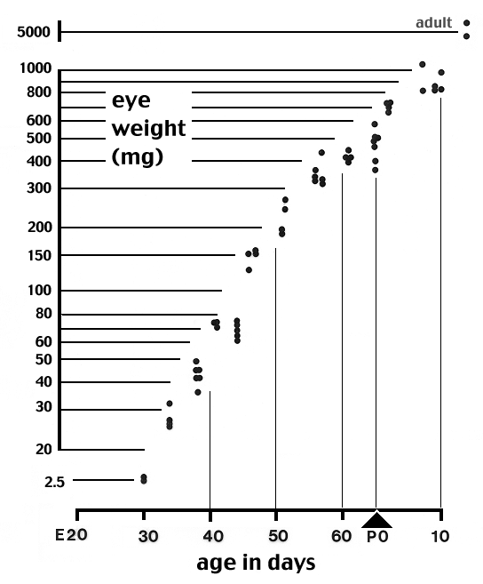
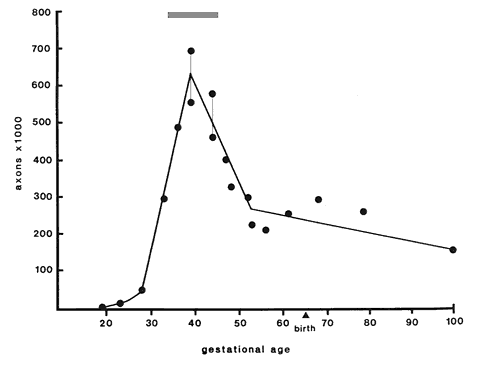
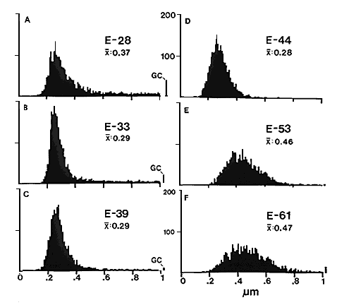
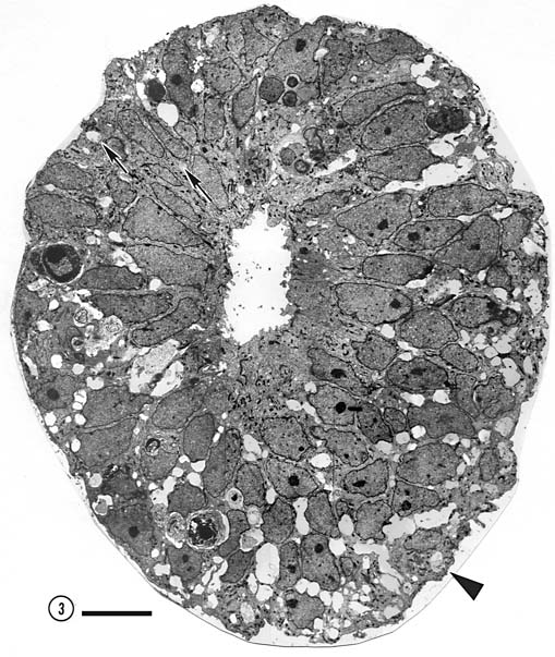
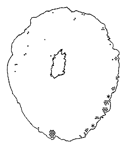
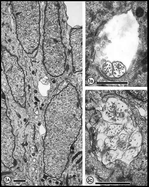
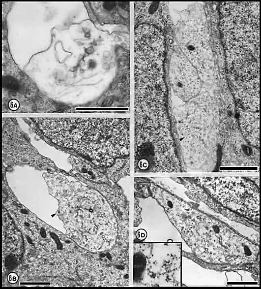
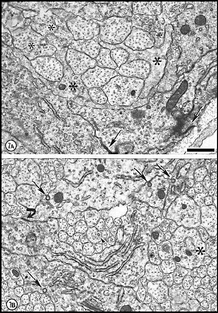
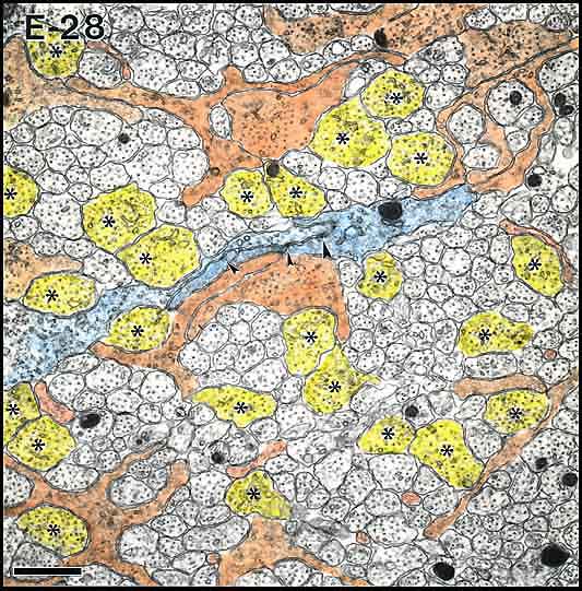
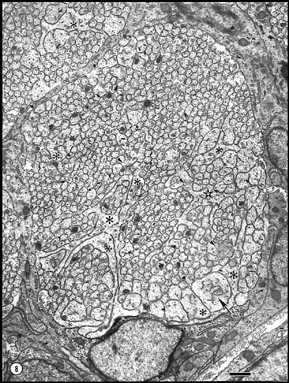
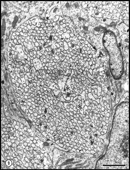
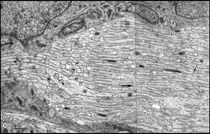
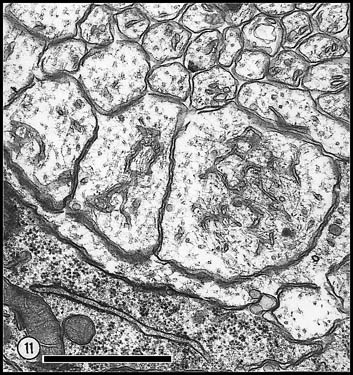

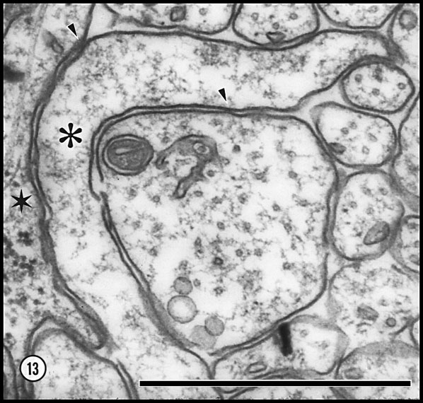

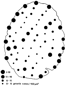
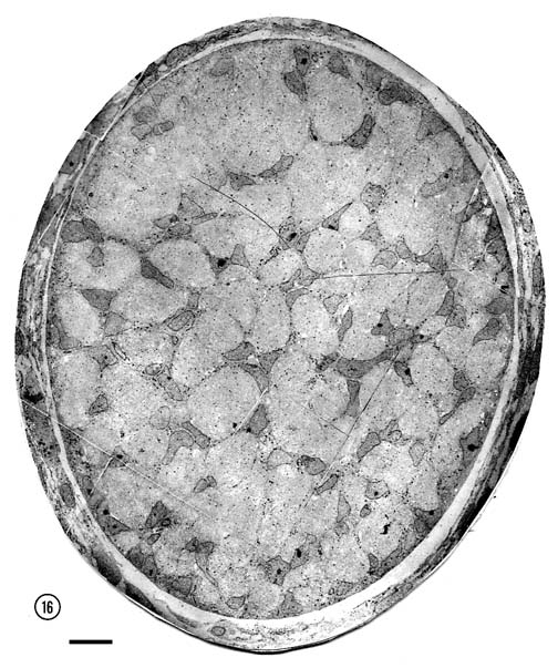
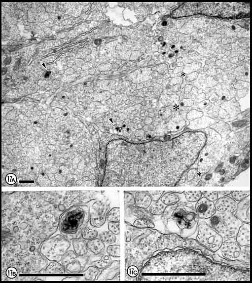
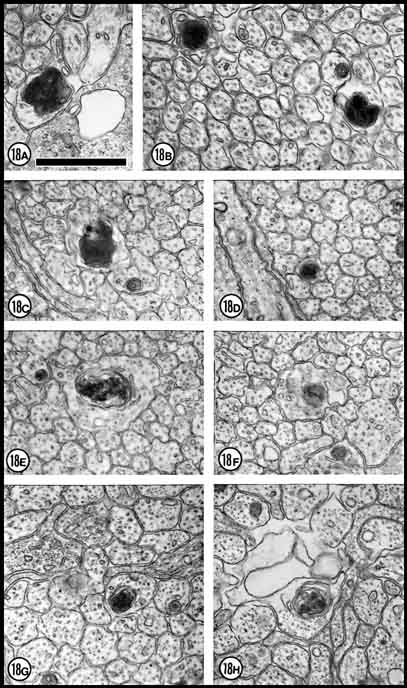
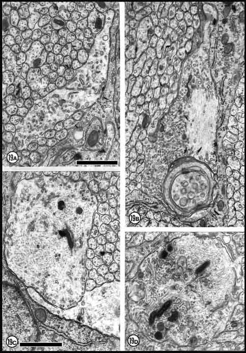
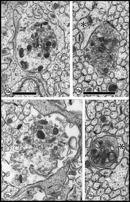
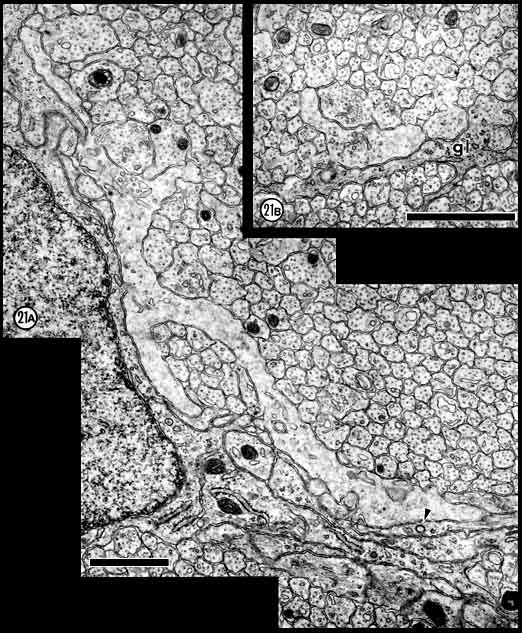

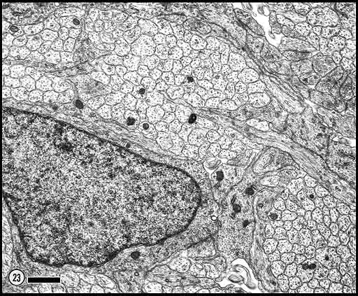
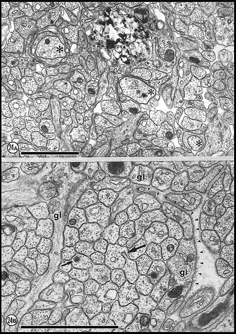
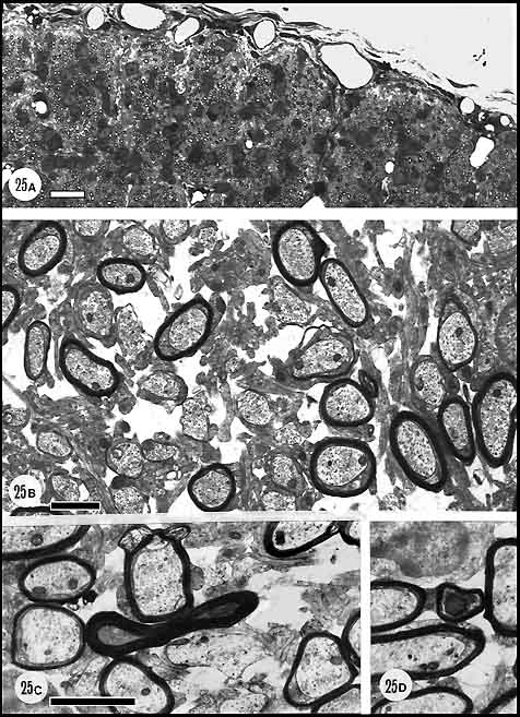


Neurogenetics at University of Tennessee Health Science Center
| PDF version | Top of Page |
Mouse Brain Library | Related Sites | Complextrait.org
