 |
| |||||
|
| ||||||||
|
| ||||||||
Home  Publications Publications |
|
|
Note to the Reader Please refer to: Williams RW, Rakic P (1988) Three-dimensional counting: An accurate and direct method to estimate numbers of cells in sectioned material. J Comp Neurol 278:344-352 (1988). Orginal version © 1988 Alan R. Liss, Inc. This HTML document is a substantially revised and expanded version of the original paper. Copyright © 1998 by R. W. Williams. NOTE: Brackets [...] and a font change are used to denote revisions and additions by R. Williams not found in the original publication. Please also note that the original publication contained an error in the description of the use of Gundersen's unbiased counting frame. This error is corrected in this revision and in our Erratum and Addendum. We thank H.J.G. Gundersen and V. Howard for pointing out this mistake. Updated Sept 10 1999.
Print Friendly We introduce a way to count and measure
cells in an optically defined volume of tissue called a counting box.
This method—direct three-dimensional counting (3DC)—eliminates the need
for correction factors, such as that introduced by Abercrombie (1946),
to determine the number of cells per unit volume (Nv).
Problems caused by irregular cell shape and cell size, nonrandom
orientation, and splitting of cells by the knife during sectioning are
overcome. Furthermore, 3DC is insensitive to large variations in section
thickness. Neuron number is a fundamental determinant of brain function
(Donaldson, 1895; Bok and Van Erp Taalman Kip, 1939, Frankhauser et al.,
1955; Vernon and Butsch, 1957; Jerison, 1963, reviewed in Williams and
Herrup, 1988). Even a small deficit of these cells can have long-lasting
effects on behavior, primarily because neurons, unlike most other cell
types are unable to proliferate throughout life (Sidman, 1970; Rakic,
1985a,b). Systematic changes in neuron number also appear to fine-tune and
balance connections between different parts of the brain and body during
normal development (reviewed in Prestige, 1970; Hamburger and Oppenheim,
1982; Cowan et al., 1984; Finlay et al., 1987). While progress in
understanding the control of neuron number has been rapid during the past
decade, a serious problem has limited the scope of studies. This problem
has to do with the methods that are used to determine the numerical
density of cells in material that has been sectioned (reviewed in Agduhr,
1941; Konigsmark, 1970; Colonnier and Beaulieu, 19985; Haug, 1986). Even
the most rigorous studies can rarely claim precision greater than ± 10%.
Consequently, only marked changes or effects can be analyzed with
confidence. Problems that demand greater accuracy and reliability cannot
be resolved with current methods. We present 3DC as an alternative to the counting method developed in the 1940s by Floderus (1944) and Abercrombie (1946, full text available). To appreciate the advantages of 3DC we begin by critiquing five features of Abercrombie's method—specifically, method 1 of the 1946 paper. Consider a section of tissue 10 µm thick. The microscopist focuses up and down through the section counting cells that fall in a 50- by 50-µm square and an average of half of those that intersect its edges (Figs. 1, 2). The group of cells that are counted includes entire cells embedded in the section and fragments of cells that were split by the knife during sectioning. The cell fragments at the upper and lower surfaces of the section are counted as it they were entire cells so that the count is always an integer. An unwelcome side-effect is that the count is too high. This is the split cell error. The thinner the section and the larger the cells, the greater the overestimate. Abercrombie (1946) reasoned that the true number of cells should equal the number of cells and cell fragments that are counted times a correction factor equal to the ratio of the section's thickness divided by the sum of the section's thickness plus the mean height of the cells: number = count x (section thickness)/(section thickness + cell height) If cells have an average height of 10µm thick, then the correction factor is 0.5 and the true number is roughly half the count. Unfortunately, there are fundamental problems that undermine the usefulness and accuracy of this correction and its variants (Floderus, 1944; Konigsmark, 1970). Some of these problems were highlighted by Abercrombie in his cogent and influential 1946 paper.
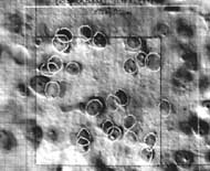
Fig. 1. A field of cells and a superimposed counting frame imaged using video-enhanced differential interference contrast (DIC) optics on a television monitor. A x100 oil immersion objective with a numerical aperture of 1.25 was used to examine this field of cells in layer V of primary visual cortex of a fetal rhesus monkey. The perimeters of several neurons in the counting box (50 by 50 by 25 µm deep) have been outlined by using a drawing program [MacMeasure] and a digitizing tablet. Some of the outlines correspond to cells not currently in the focal plane. [A QuickTime movie of a through-focus series of DIC images used for 3DC is available.] The first problem is that the method is biased (Abercrombie, 1946; Marrable, 1962; Aherne, 1967; Konigsmark, 1970; Hendry, 1976). Systematic errors will arise if the size, shape, and orientation of cells are not taken into account (Snedecor and Cochran, 1980; Cruz-Orive and Hunziker, 1986). It is difficult to determine how much bias different methods generate (Marrable, 1962; Colonnier and Beaulieu, 1985). Abercrombie warned that his method would tend to overestimate cell number by 5–10%. The problem of bias becomes more serious and less predictable when the size distribution of cells is skewed or bimodal (Hendry, 1976).
Fig. 2. A schematic of a counting frame, ABCD, that defines the length and width of the counting box—50 µm in both dimensions. This counting frame is a cross section through the counting box shown in Figure 3, as viewed from the top. Thus, corner A in this figure matches the back left edge of the counting box in Figure 3. The unshaded cells are counted; the shades cells are excluded. The three-dimensional positions of cells in this figure are shown schematically in Figure 3. [The asterisk in the lower right corner is intended to highlight the correction made to the original figure in which line segment DC was extended through cell 7 to the right of the page. This was incorrect, and as shown in this revised figure, the line is actually reflected downward at point C.]
Fig. 3. A counting box. This schematic shows a small piece of tissue cut at a nominal thickness of 40 µm. The thickness actually varies ± 4 µm. The counting box has dimensions of 50 x 50 x 25 µm and is embedded entirely within the section. It is insulated from the rough-cut surfaces of the section by upper and lower guard zones. Thus, cells cut in half by the knife (e.g., the cell labeled cut), and the cells that are torn away from surrounding tissue (cell labeled not cut and the pit left by a cell torn away with the adjacent section) do not compromise the accuracy of the counting procedure. The same cell outlines shown in Figure 2 are depicted here positioned in three dimensions. Applying the counting rules gives the following results: Cells 11-14, which are completely inside the box, are counted. Cells 1 and 8-10, which cross through the forbidden planes are excluded [Cell 7 should be included]. The transections of these cells with the forbidden planes are shaded. Note that the forbidden planes extend outward in Figure 2. For this reason cell 1 in the upper left corner of the box is excluded. Similarly, the bottom forbidden plane extends across the entire section. Cells 2, 4, and 5 only cross the top, right, and back sides, and, therefore, are included in the count. [In the original publication we stated that cell 7 in the lower right corner should not be counted. This cell should actually be counted. Our erratum and addendum explains more completely why cell 7 should be counted, and see Figure 2.] The second problem is the difficulty of determining an appropriate
value for object height to enter into the equation. Abercrombie's
impractical solution was to measure the diameter of cells in sections cut
precisely at right angle to the remainer of the tissue. In practice, this
is almost never done. [But see Abercrombie and Johnson, 1946, J. Anat.
Lond. 80:37-50; for an example.] Instead, cell diameter is substituted for
cell height. In some cases, for instance, when cells are oblong or when
the tissue shrinks unevenly during processing, the differences between
these two measurements can be substantial. Method and ImplementationThe essential feature of a 3DC system is that it accurately defines a small volume of tissue called a counting box (Fig. 3). A key feature of 3DC is that the top and bottom sides of the counting box are inside the section, a precisely defined distance away from the cut surfaces of the section. When the counting box has been set up, cells in and around the box are counted by using the rules listed below:
Defining the counting boxThe four walls of a counting box are defined by using a counting frame or an eyepiece reticle. As the tissue is moved up and down through the focal plane, the edges of the frame trace out the walls. When a video monitor is used for counting, a plastic frame can be placed directly on the screen, or a frame can be generated and displayed by using a computer (Fig. 1). The top and bottom sides of the counting box are defined using a shaft encoder or a length gauge. Ideally, the accuracy and resolution of these devices should equal the depth of focus of the objective. A shaft encoder has the advantage of being inexpensive but the disadvantage that measurements are indirect: rotation of the fine-focus control is measured, not vertical movement. For this reason, it is necessary to calibrate the linearity, accuracy, and thermal stability of the focusing mechanism throughout its range.1 A digital length gauge does not have this problem. The tip of the gauge rests on the stage. Measurements are direct and calibration of the focus control is not necessary. Resolution of 0.1 µm and accuracy of 0.2-0.5 µm can be achieved with either method. Footnote 1. There are no commercially available vertical calibration standards for transmitted light microscopy. We have constructed our own standard by using 0.25- and 0.48-thousandth-of-an-inch Mylar plastic sheets calibrated with a length gauge to an accuracy of better than 0.2 µm. [Including calibrated microspheres in embedding medium or tissue, may be an alternate method.] Signals from the shaft encoder or the digital length gauge are decoded
and displayed using a Z-axis control unit. This custom-made unit has two
programmable relays that trigger high and low frequency tone generators.
The vertical positions at which tones are produced correspond to the top
and bottom sides of the counting box. As a result, deciding whether a cell
is inside the counting box, above or below the box, or crosses through the
top or bottom side of the box is simple and can be done without having to
look away from the monitor. An alternative method of defining the top and
bottom sides of the counting box is to use the relays to change the color
background of the monitor. This can be done with an RGB monitor by using
the two relays to interrupt the red and green video signals.
Optical height vs. true heightThe accuracy of the 3DC method depends on the precision with which the height of the counting box is defined. The measured height of objects imaged with a microscope depends on differences in the refractive indices of the tissue, the objective, and the material in which the tissue and slide are immersed (Snell's law of refraction). If a dry objective is used to focus first on the top and then on the bottom of an object, the distance the stage travels will only be 66% of the true distance separating the top and bottom (Galbraith, 1955; Glaser, 1982; Gahm and Witte, 1986). The difference is accounted for by the ratio of the refractive indices of air and crown glass (1.000:1.524). An object that is 45 µm high will be imaged over a vertical distance of only 30 µm. Obviously, when one uses dry objectives, refraction must be taken into account in order to define the height of a counting box. The Z-axis control unit we have built can compensate for such optical foreshortening. A much better solution is to avoid this problem by using oil immersion. When an oil immersion objective is used, the tissue, the mounting medium, and coverglass, the immersion oil , and the glass of the objective have refractive indices very close to 1.52 ± 0.02 (Emil, 1943; Loveland, 1981, pp. 64, 65). Thus, the optical height and the true height of objects correspond almost exactly. 2 Footnote 2. The refractive index of living tissue is substantially lower than that of dead or fixed tissue (Gahm and Witte, 1986) and consequently measurements taken from living tissue will be foreshortened by about 9%.
Depth of fieldUltimately, the depth of field limits the minimum height of a counting box. If the box is 2 µm high and the depth of field is 0.5 µm, it will not be possible to determine with precision the vertical position of cells with respect to top and bottom sides. The depth of field of an objective depends on its [effective] numerical aperture (NA), the wavelength (L) of light (about 0.55 µm), and the refractive indes (ri) of immersion oil (Beadle, 1940; Loveland, 1981; his appendix 1):
The higher the aperture of the lens, the shallower the depth of field. The depth of field of an oil objective with a [realized] NA of 1.4 is 0.16 µm. A section that is 6 µm thick can be sectioned optically into 20–40 levels. It is, therefore, possible to determine accurately which cells cross through the top and bottom sides of the counting box. Infrequently, however, errors will be made at these sides. For instances, cells above the box may have very small polar segments that extend through the top side of the box. If these small polar segments are not detected, the cells will not be counted (Floderus, 1944; Konigsmark, 1970). Such errors of omission will be counterbalanced somewhat by errors of commission made at the bottom side of the counting box. These counterbalancing errors are generated by cells that are included in the count even though they have polar segments that extend through the forbidden bottom surface of the box. To reduce any possible asymmetry in the incidence of the errors at top and bottom sides of the box due to the finite depth of focus or to the polar caps, one can switch the relative roles of the top and bottom sides of the counting box and average the two resulting counts. In practice, we have never found this necessary. [It is sometimes important to coverslip the relatively thick sections used for 3DC using the thinner Number 1 (1 ounce) coverslips. These have a thickness of less than 130 µm. This makes it possible to focus on the bottom of thick sections even when using high NA objectives that have modest working distance (90 µm). If you use 1.5 ounce coverslips you may not have sufficient working distance to define a couting box. However, note that most dry objectives are designed for minimal spherical aberration when used in conjunction with the 1.5 ounce coverslips].
Section thicknessThe fourth problem we pointed out with Abercrombie's correction is its
sensitivity to variation in the thickness of sections. 3DC largely
overcomes this problem (Fig. 3). The height of the counting box is fixed
by the investigator—not by idiosyncratic interactions between the block of
tissue and the knife. The counting box is insulated from variation in
section thickness that occur during sectioning by the guard zones that lie
above and below the box (Fig. 3). Ideally, the guard zone above the top
side of the counting box should be higher than the largest cells. Cells
that cross through the top side of the box are potentially included in the
count, so it is important that they can be identified unambiguously, if
necessary, by focusing above the top side. If the guard zone is thick
enough, 3DC will be immune to the fifth problem—cell identification. In
practice, the guard zone may be shorter than the height of the largest
cells. For instance, nuclei of neurons often have a simple, nearly
spherical shape and can be distinguished easily from glia and pericytes
(Williams and Rakic, 1988). As a result, in many cases the upper guard can
be safely set at one-half the height of the larger cells or nuclei: 4 µm
is adequate. The lower guard zone can always be shallow (often less than 2
µm), because all cells or other objects that intrude into this zone are
excluded from the count (Fig. 3). Identification is not an issue. [Special caution applies to the analysis of frozen-sectioned
material. Frozen tissue cut at 50 µm that is mounted on a gelatinized
slide will shrink in thickness to 20 µm or less when dehydrated through
alcohol and xylene (a residual thickness of merely 10 µm is not uncommon).
There is no guarantee that this shinkage will be uniform, particularly if
tissue is processed rapidly. Tissue close to the exposed surface may
shrink more than tissue close the glass. If the counting box is
consistently defined in a region with greater or lesser shrinkage, then
systematic bias may be introduced. There may also be substantial
section-to-section and batch-to-batch variation in frozen section. As a
result, the effective volume of the counting box may be quite variable. (RW
June 1998)
Reasons for differential interference contrast (DIC) opticsIt can be difficult to get high-definition images from thick sections. To increase contrast and definition and improve the vertical resolution of images we recommend using DIC optics. With this method it is easy to decide whether the edges of cells or nuclei extend beyond the boundaries of the counting box (Fig. 1). Furthermore, at high magnification, unstained or weakly stained tissue can be readily counted. DIC optics offer another significant advantage: the iris diaphram of the condenser can be opened to match teh NA of the objective. This gives the best possible resolution and a narrow depth of filed without loss of contrast (Inoué, 1986, pp. 122-133). If fluorscent cells are to be counted, it may be necessary to reduce out-of-focus blur by using an image procesor or confocal optics. [DIC optics greatly improve the effective Z-axis resolution of a bright-field microscope. By stripping away low spatial frequencies and by enhancing high spatial frequencies, the definition of all boundaries is greatly improved. This is true even when imaging conventional Nissl-stained tissue. DIC optics may cost $6,000 to $12,000, but it is well worth the expense. An excellent but more costly alternative, particularly when counting fluorescently labeled cells, is to use an optical or digital confocal microscope system]
Count accuracy and video mixingCurcio and Sloan (1986) point out that a major deterrent to the use of
quantitative methods is the"difficulty, tedium, and human error often
associated with analysis of the large tissue samples necessary for
statistically useful conclusions." In our experience, counts made directly
at the microsope through the eyepiece are often in error by one or two
cells in a frame of merely 20 cells (5-10% error). This error is also
systematic; counts are almost invariably low. This problem is even more
serious when thick sections are counted. Not only can the number of cells
in a counting box be high (>50), but cells are often stacked on top of
each other. Accuracy can be improved signficiantly by marking cells as
they are counted. We used a video/computer mixing system to do this. The
computer/video mixer is not an essential part of the 3DC system, but after
having used such a system we would never consider reverting to counting at
the eyepiece. The computer/video system improves speed and accuracy and
reduces fatigue.
Quality of the video imageWe have used a Newvicon video camera that has a central resolution of 700 scan lines. The image is displayed on a monitor with with comparable resolution (see Inoué, 1986, for a lucid discussion of video systems and the measurement of video resolution). Given the magnificiation of the image projected onto the facplate of the camera, a scan line corresponds to a 0.15-µm-wide strip of tissue, and consequently the system can resolve objects separated by a distance of about 0.4 µm (twice the equivalent scan width divided by the Kell factor of 0.7; Inoué, 1986). The great advantage of the video system is the ability to adjust the contrast and brightness of the image by using a video processor. With DIC optics, sharp images can be obtained from poorly and unevenly stained specimens.
Step-by-step counting procedureIn this section we give an example of the steps we use to determine the volumetric cell density and absolute cell number. Step 1. We start by measuring the thickness of several sections. Based on these measurements and their variation we decide what height the counting box should be. If the sections are between 36 and 44 µm thick, then to define a box with a height of 25 µm, we set one relay to trigger 3 µm above the bottom surface of the section and the other relay to trigger 28 µm above the bottom surface of the section. In this particular example, the lower guard zone will be 3 µm thick at all sites in all sections, while the height of the upper guard zone will vary in thickness from 8 to 16 µm. Step 2. We next adjust the length and width of the counting box. This will depend on the sampling strategy and one the density of cells (Snedecor and Cochran, 1967, Chapter 21; Gundersen, 1981)3. Footnote 3: Parts of the brain with steep gradients in cell density—retina, for instance, with its 50-100 fold regional differences (Lia et al., 1987)—are particularly difficult to deal with an require a stratified sampling protocol. Parts of the brain with lesser gradients may be sampled adequately by using a simple procedure. In cases in which a laminate structure is to be counted (e.g. the dorsal lateral geniculate nucleus, the optic tectum, or a part of the cortex), a series of adjacent counting boxes that extend fully across the laminae should be analyzed, and this series of boxes should then be treated as a single, but large, counting box. Step 3. Before making and counting cells, we focus on the lower surface of the section at the particular site and reset the Z-axis control unit to zero. We confirm that the relays trigger at the correct vertical levels and that the slide is not drifting. It is usually necessary to reset the zero position when the slide is moved laterally. Step 4. We begin counting by marking all cells that are completely inside the box. As each cell is marked, the computer counts it. We typically count cell nuclei rather than cell bodies or nucleoli. The edges of nuclei are more distinct than the edges of cell bodies. And in contrast to nucleoli, there is one and only one nucleus per cell in the nervous system. We mark nuclei by tracing their perimeters. Step 5. We next mark and count all cells that extend beyond the counting box but that do not cross through the lines that define the left and bottom edges of the counting frame (see Figs. 1, 2). We do this while moving the focus back and forth from top to bottom. If a cell crosses over one of these two forbidden lines but at a level above the top of the counting box then it still must be excluded (for instance, cell 1 in Figure 3). Step 6. Finally, we mark and count cells that cross the top surface of the counting box. These are the cells that are visible when the high tone is first generated by the Z-axis control unit. Step 7. We divide the total count (the sum of steps 4 to 6) by the volume of the counting box. This gives us an unbiased estimate of the local cell density, Nv. Step 8.We repeat steps 4 to 6 at different sites and calculate the 95% confidence interval of the mean of the measurement of Nv. This value is a conservative estimate of the precision of the average cell density and does not take into account systematic regional differences. To get a more precise estimate of the confidence interval, it may be necessary to perform a regression analysis (Snedcor and Cochran, 1967, pp. 186, 444-446.) Step 9. We estimate the total cell number by multiplying the mean density by the total volume of the region in which the counting boxes were distributed.
Fig. 4. A typical setup for direct 3DC. On the left side of the figure, a microscope is shown equipped with a shaft encoder (Hewlett-Packard HEDS-6000B-06) on the fine-focus control, and a digital length gauge (Heidenhain Metro-25 digital length gauge; Heidenhain Corp., Elk Grove Village, IL) is shown positioned over the stage. Only one of these sensing devices is required. The Z-axis control unit decodes and displays the vertical position of the stage with a resolution of 0.1 µm and generates high and low tones when the stage moves above or below the top and bottom sides of the counting box. The video mixing equipment includes a video camera, a video processor, a video mixer, and a television monitor.
Using 3DC to measure cell sizeIt is often useful to determine the size distribution of cell
populations. This can be hard, particularly when an unbiased sample of
cells cannot be selected easily. To overcome this problem, the 3DC
counting rules can be applied. The unbiased sample of cells is then
measured. In many cases, it is useful to determine mean cell diameter.
Typically, the focus is adjusted until the cross-sectional area of each
cell reaches a peak. The perimeter of this near-equatorial transection is
traced and the area is computed. This measurement is converted to the
'equivalent' diameter—the diameter of a circle that has the same area as
the cell's equatorial transection. The distribution of a set of these
measurements gives an unbiased and direct estimate of cell size in the
image plane.
DiscussionGiven the level of interest in neuron number and its control, it is surprising how little solid information we have (reviewed in Blinkov and Glezer, 1968). The most obvious reason for this is that research is hampered by serious methodological problems. Estimating absolute numbers of neurons and rates of change in neuron populations is difficult, usually imprecise, and is the worst cases, even subjective. While the number of neurons in the nervous systems of several species of coelenterates, nematodes, and annelids is known with precision (Bullock and Horridge, 1965), estimates in vertebrates are often woefully inaccurate (reviewed in Jones, 1937; Agduhr, 1941; Blinkov and Glezer, 1968; Konigsmark, 1970; Haug, 1986; Peters, 1987; Williams and Herrup, 1988). And as a rule, the larger the brain, the greater the margin of error. For instance, estimates of the number of neurons in the human brain have an almost absurd range—from 10 billion to 1 trillion. This problem is not a minor impediment that prevents us from solving trivial problems in brain statistics and cell demographics. It is a major barrier that blocks our way to a better understanding of the development, function, pathology, and evolution of the nervous system—both at descriptive and mechanistic levels.
Fig. 5. Citation frequency of Abercrombie's 1946 paper in neuroscience journals (gray bars) and in all other journals (black bars). These data were extracted from the Science Citation Index, Institute of Scientific Information, Inc., 1955-1987. Roughly 500 of the 1,205 citations listed in the index were published in The Journal of Comparative Neurology, the largest number for any journal. The incidence of miscitation of Abercrombie's paper is high. For example, the first page number is given incorrectly by more than 133 (11%) of the papers.[Ironically, even this paper (Williams and Rakic, 1988) miscited the title of Abercrombie's paper: the correct title is Estimation of Nuclear Population from Microtome Sections. Despite significant drawbacks, Abercrombie's Method 1 (1946) continues to gain adherents and influence. The 1946 paper is one of the most widely cited publications in science, with a total of more than 1,200 citations (Fig. 5). Even more impressive, the rate of use of this particular correction has increased greatly in the past few years: the paper is more cited 100 times a year. Evidently the method's practicality has outweighed its problems. In this paper we have described an equally practical, more accurate, and more reliable way to determine cell number. Each of the five problems that we raised with Abercrombie's method are overcome. The reduced effort and improved accuracy more than offset the modest investment in equipment.
Precedents of 3DCThe first suggestion that an ideal way to count cells would be to keep
track of their three-dimensional position in sectioned material was made
by T.W. Blackstad in a discussion appended to Konigmark's well-cited
review (1970). Blackstad suggested that a microscope developed by Glaser
and Van der Loos (1965) capable of encoding the position of cells in three
dimensions could be used to obtain direct estimates of cell number: "I can
easily imagine myself doing the identification (of neurons and glia) and
feeding the X-Y-Z coordinates of each cell into a computer, going through
the entire, length, wide, and depth of the tissue section." The 3DC system
we have developed accomplishes Blackstad's goal, but instead of
determining the precise three-dimensional positions of cells, we define
the position of six sides of a counting box and then simply mark and count
cells in and around the box.
Practicality of 3DCCounting is tiresome. It is no surprise that an accurate but difficult method will not be used. In comparison to Abercrombie's method and its variants (Konigsmark, 1970), 3DC is simple. It is less work because cell size is not a factor and therefore does not need to be measured, and the data do not have to be corrected (Hendry, 1976) 3DC, however, does involve a more complex counting procedure. Cells must be categorized in relation to the counting box and its sides. However, the added effort is not significant and is offset by improved reliability and accuracy. The hardware requirements of the 3DC system, summarized in Figure 4, are modest. The only equipment that is dedicated to the system is the Z-axis control unit and the position encoder.
Applicability of 3DCOne limitation of our method is that sections must be thick enough to accommodate a counting box that is substantially thicker than the depth of field of the objective. We recommend that sections be at least 6-8 µm thick. At the other extreme, there is not theoretical limit. The upper parts of slabs of tissue, 100 to 250 µm thick, can still be counted if they can be imaged. The depth to which the counting box can extend into the section will, however, be limited by the working distance of the objective.
Accuracy of 3DCThree main factors determine the accuracy of an estimate of cell number:
Up until now the weak link in determining total cell number in a
particular part of the nervous system has been the method used to
determine Nv. The direct three-dimensional
method strengthens this link. The counting protocol makes no assumptions
about cell size, shape, or orientation (Gundersen, 1977; Howard et al.,
1985). Consequently, a correction is not required. This is why we call 3DC
a direct and inherently accurate method.[While a local estimate of Nv
may be "technically" unbiased, this does not mean that the final estimate
for an entire tissue will be unbiased. Tissue preparation, poor staining
or counting, differential shrinkage and compression, and numerous other
factors can introduce bias into regional density estimates and final cell
counts.] (RW Sept 99)
Absolute vs. comparative accuracy of 3DC
In many other situations, absolute cell number does matter. Absolute
cell number, unlike numerical density, is in theory independent of the
method used to process the material. However, the inaccuracy of current
counting methods has meant that even absolute numbers cannot be given much
weight. Consequently, it has been difficult to confirm or refute results.
Differences in absolute numbers may hinge on the relative merits of
corrections. Certainly if we want to compare sets of data, the accuracy
with which we can estimate absolute cell numbers is crucial.
AcknowledgementsThis research was supported by grant EY-0293 (to PR) and EY-06627 (to
RW). We thank Dr. Kenneth C. Wikler for comments on this paper. We thank
Richard H. Moore of du Pont Co. for samples of Mylar and Jan Hinsch of E.
Leitz, Inc. and Martin Scott of Eastman Kodak Co. for valuable suggestions
that helped us refine the 3DC system. [Support for this revised version
provided in part by NS 35485 (to RW).]
ReferencesAbercrombie, M. (1946) Estimation of nuclear population from microtome sections. Anat. Rec. 94:239-247. Agduhr, E. (1941) A contribution to the technique of determining the number of nerve cells per volume unit of tissue. Anat. Rec. 80:191-202. Aherne, W. (1967) Methods of counting discrete tissue componenets in micrscopical sections. J. R. Microsc. Soc. 87:493-508. Bok, S.T., and M.J. Van Erp Taalmann Kip (1939) The size of the body and the size oand the number of nerve cells in the cerebral cortex. Acta Neerl. Morphol 3:1-22. Braendgaard, H., and H.J.G. Gundersen (1986) The impact of recent stereological advances on quantitative studies of the nervous system. J. Neurosci Methods 18:39-78. Clarke, F. (1967) A comparative analysis of methods of estimating the size of cell populations from microtome sections. J. R. Microsc. Soc. 88:18-03. Colonnier, M., and C. Beaulieu (1985) An empirical assessment of stereological formulae applied to the counting of synaptic disks in the cerebral cortex. J. Comp. Neurol. 231:17-79 Cowan, W.M., J.W. Fawcett, D.D.M. O’Leary, and B.B. Stanfield (1984) Regressive events in neurogenesis. Science 225:125-265. Cruz-Orive, L.M. (1986) Particle number can be estimated using a disector of unknown thickness. The selector. J. Microsc. 145:12-42. Cruz-Orive, L.M., and E.B. Hunziker (1986) Stereology for anisotropic cells: Application to growth cartilage. J. Microsc. 143:4-0. Curcio, C.A., and K.R. Sloan, Jr. (1986) Computer-aided morphometry using video-mixed microscopic images and computer graphics. Anat. Rec. 214:32-37. de Groot, D.M.G., and E.P.B. Bierman (1986) A critical evaluation of methods for estimating the numerical density of synapses. J. Neurosci. Methods 18:7-01. Donaldson, H.H. (1895) Growth of the Brain: Study of Nervous System in Relation to Education. New York: Scribner. Fankhauser, G., J.A. Vernon, W.H. Frank, and W.V. Slack (1955) Effect of size and number of brain cells on learning in larvae of the salamander, Triturus viridescens. Science 122:69-93. Finlay, B.L., K.C. Wikler, and D.R. Sengelaub (1987) Regressive events in brain development and scenarios for vertebrate brain evolution. Brain Behav. Evol. 30:10-17. Floderus, S. (1944) Untersuchungen über den Bau der menschlichen Hypophyse mit besonderer Berücksichtigung der quantitativen mikromorphologischen Verhältnisse. Act Pathol. Microbiol. Scand. [Suppl.] 53:-76. Galbraith, W. (1955) Optical measurement of depth. Q. J. Micro. 96:28-89. Gahm, T., and S. Witte (1986) Measurement of the optical thickness of transparent tissue layers. J. Microsc. 141:14-10. Glaser, E.M., and H. Van der Loos (1965) A semi-automatic computer microscopy for the analysis of neuronal morphology. IEEE Trans. Biomed. Eng. BME 12:2-1. Glaser, E.M. (1982) Snell’s law: The bane of computer microscopists. J. Neurosci. Methods 5:20-02. Graf, W. (1948) The microtome as an error producing factor in quantitative histological investigations. Acta Anat 6:14-44. Gundersen, H.J.G. (1977) Notes on the estimation of the numerical density of arbitrary profiles: The edge effect. J. Micros. 111:21-23. Gundersen, H.J.G. (1986) Stereology of arbitrary particles: A review of unbiased number and size estimators and the presentation of some new ones. J. Microsc, 143:-5. Gundersen, H.J.G. and E.B. Hensen (1986) The efficiency of systematic sampling in stereology and its prediction. J. Micros 147:22-63. Hamburger, V. and R.W. Oppenheim (1982) Naturally occurring neuronal death in vertebrates. Neurosci. Commmun. 1:3-5. [Hatton, W.J. and C. S. von Bartheld (1999) Analysis of cell death in the trochelar nucleus of chick embryos: calibration of the optical disector couting technique reveals systematic bias. J. Comp. Neurol. 409:169–186.] Haug, H. (1986) History of neuromorphometry. J. Neurosci. Methods 18:-7. Hendry, I.A. (1976) A method to correct adequately for the change in neuronal size when estimating neuronal numbers after growth factor treatment. J. Neurocytol. 5:33-49. Howard, V., S. Reid, A. Baddeley, and A. Boyde (1985) Unbiased estimation of particle density in the tandem scanning reflected light microscope. J. Microsc 138:20-12. Inoué, S. (1986) Video Microscopy. Plenum Press. New York. Jerison, H.J. (1963) Interpreting the evolution of the brain. Hum. Biol. 35:25-91. Jones, R.L. (1937) Split nucleoli as a source of error in nerve cell counts. Stain Technol. 12:9-5. Konigsmark, B.W. (1970) Methods for counting of neurons. In. W.J.H. Nauta and S.O.E. Ebbesson (eds): Contemporary Research methods in Neuroanatomy. New York: Springer-Verlag, pp. 31-40. Lia, B., R.W. Williams, and L.M. Chalupa (1987) Formation of retinal ganglion cell topography during prenatal development. Science 236:84-51. Loveland, R.P. (1981) Photomicroscopy. A Comprehensive Treatise. Reprint with New Appendices. Malabar, Florida: Krieger. Marrable, A.W. (1962) The counting of cells and nuclei in microtome sections. Q. J. Microsc. Sci. 103:33-47. Peters, A. (1987) Number of neurons and synapses in primary visual cortex. In E.G. Jones and A. Peters (eds): Cerebral Cortex. Vol. 6. New York: Plenum, pp. 26-94. Prestige, M.C. (1970) Differentiation, degeneration, and the role of the periphery: quantitative considerations. In F.O. Schmitt (ed): The Neurosciences, Second Study Program. New York: Rockefeller Univ. Press, pp. 7-2. Rakic, P. (1985a) Limits of neurogenesis in primates. Science 227:105-056. Rakic, P. (1985b) DNA synthesis and cell division in the adult primate brain. Ann. NY Acad Sci. 457:19-11. Rose, R.T., and D. Rohrlick (1987) Counting sectioned cells via mathematical reconstruction. J. Comp. Neurol. 263:36-86. Sidman, R.L (1970) Autoradiographic methods and principles for study of the nervous system with thymidine-H3. In W.J.H. Nauta and S.O.E. Ebbesson (eds): Contemporary Research Methods in Neuroanatomy. New York: Springer-Verlag, pp. 25-74. Snedecor, G.W., and W.G. Cochran (1980) Statistical Methods. 7th ed. Ames, Iowa: Iowa Univ. Press. Sterio, D.C. (1984) the unbiased estimation of number and sizes of arbitrary particles using the disector. J. Microsc 134:12-36. Vernon, J.A., and J. Butsch (1957) Effect of tetraploidy on learning and retention in the salamander. Science 125:103-034. [von Bartheld, C.S. (1999) Systematic bias in an "unbiased" neuronal counting technique. Anat Rec 257:119–120.] Williams, R.W., and P. Rakic (1986) Pronounced architectonic differences between monocular and binocular segments of the monkey’s striate cortex. Soc. Neurosci. Abstr. 12:1498. Williams, R.W., K. Ryder, and P. Rakic (1987) Emergence of cytoarchitectonic differences between areas 17 and 19 in the developing rhesus monkey. Soc. Neurosci. Abstr. 13:1044. Williams, R.W., and K. Herrup (1988)The control of neuron number. Annu. Res. Neurosci. 11:42-53. Williams, R.W., and P. Rakic (1988) Elimination of neurons from the rhesus monkey’s lateral geniculate nucleus during development. J. Comp. Neurol. 272:42-36.
Since 11 August 98
|
Neurogenetics at University of Tennessee Health Science Center
| Print Friendly | Top of Page |
Mouse Brain Library | Related Sites | Complextrait.org
