 |
| |||||
|
| ||||||||
|
| ||||||||
Home  Publications Publications |
|
|
Note to the Reader This is a revised edition of a paper published in Seminars in Cell and Developmental Biology. The definitive original print version is available from Academic Press and on-line at the Idealibrary at http://www.hbuk.co.uk/ap/journals/sr.htm. New figures, text, and links have been incorporated into the revision. Revised HTML (http://www.nervenet.org/papers/RetinaRev98.html) copyright ©1999 by Robert W. Williams Seminars in Cell & Developmental Biology (1998) 9:249–255.
Print Friendly Genetic Analysis of
Retinal Ganglion Cells Retinal development depends on complex interactions between products
of thousands of genes and numerous cellular and environmental factors.
We are using novel quantitative genetic methods to map and characterize
genes that are responsible for the pervasive quantitative differences in
the architecture of the eye and the retina. These genes, known as
quantitative trait loci (QTLs), may also determine susceptibility to
common eye diseases. To map QTLs that generate variation among normal
individuals we have analyzed several traits in a wide variety of mice,
including standard inbred strains, recombinant inbred strains, wild
mice, F1 hybrids, and intercross progeny. Here we review this approach
and give three specific examples of how genes with well-defined
functions in retinal development are being mapped and characterized. Retinal cDNA libraries contain more than 15,000 transcripts generated
from as many as 10,000 genes. Half of these genes may have common roles
in cellular metabolism, but the other half contribute more specifically
to retinal development and function. Understanding how such large
populations of genes interact with each other and with many exogenous
factors to generate and maintain the retina is a major intellectual
challenge, but there are reasons for optimism. Techniques are advancing
rapidly and progress is being made in tracing the intertwined molecular
and cellular pathways of eye development. Within twenty years we can
anticipate having sophisticated databases of gene expression in
individual retinal cell types. We may, for example, know when
differences in gene expression first distinguish ON- and OFF-bipolar
cells; we may know what genes contribute to the remarkable diversity of
amacrine cell phenotypes, and we may know what genes help differentiate
ganglion cells into populations with crossed and uncrossed projections. Genetics of natural variation This leaves an important area of research untouched—namely, which of
these thousands of genes generate natural variation in the retina. Which
genes contribute to the three-fold difference in cone density in the
foveal pit of humans (Curcio et al. 1987)? Which genes predispose some
of us to myopia or glaucoma? Which genes help generate variation in
ratios of rods and cones (Wikler et al., 1990)? To answer these types of
questions we need to know which genes are normally variable, and we need
to know how allelic variants produce significant differences in the
development and organization of the eye. This type of information is not
only critical in understanding sources of variation within a species,
but it is also critical in understanding the amazing variety of eyes
that natural selection has produced by relatively subtle genetic changes
(Walls, 1942; Wikler and Rakic, 1990; Williams et al., 1993). Common gene polymorphisms and rare mutations This article describes and illustrates a strategy that we are using
to answer these types of questions (Williams et al., 1996, 1998). Our
aim is to find and characterize an important set of genes responsible
for normal differences in retinal structure among mice. Almost all
heritable variation is produced by polymorphic genes—genes that have two
or more common alleles. About 10% to 20% of genes are polymorphic in
vertebrate populations (Nei, 1987; Levinton, 1988). This implies that
1000 polymorphic genes may contribute to variation in the eye and retina
within most species. Nothing is now known about these genes. Our focus
on normal variants complements the analysis of rare mutations that
disrupt retinal development. It will be important to establish if any of
the long list of mutated genes that perturb retinal development also
have normal allelic variants with more tempered effects. Mapping QTLs that generate variation of retinal architecture
Until recently, it has not been practical to dissect complex traits
controlled by large numbers of genes in vertebrates (Lander and Schork,
1994). Genome maps were sparse and genotyping was hard work. However, we
now have high density genome maps, as well as rapid and sensitive
methods that make it practical to map the quantitative trait loci (QTLs)
that generate normal variation in heritable traits. The polymerase chain
reaction (PCR) combined with gel electrophoresis is the current choice
for high-throughput genotyping, but chip-based methods that promise a
huge improvement in efficiency will dominate within a decade (Shoemaker
et al., 1996). A forward genetic approach (from traits to genes) can now
be used to map functional categories of genes from among the thousands
that are involved in retinal development. For example, it is now
possible to find specific QTLs that modulate ratios of rods and cones or
that modulate numbers of early- and late-generated retinal cell types.
We do not have to wait for a spontaneous mutation or a knockout mouse
with the right effects. We have started this type of analysis by
studying several important and easily measured traits: eye weight, total
retinal surface area, the density of horizontal cells, and the total
number of retinal ganglion cells (Williams et al.,
1996,
1998; Strom and Williams,
1998). We have begun with these traits because of their functional
significance and because they are practical to measure in large numbers
of animals. The Essence of QTL mapping Mapping a gene involves finding a pattern of allelic differences that
correspond with phenotypic differences in a set of animals (Tanksley,
1993; Lander and Schork, 1994; Williams,
1998). If every gene had two alleles (the alpha gene had alleles A+
and A–, the beta gene had alleles B+ and B–, etc.), and if all of these
genes assorted independently during the production of gametes (one gene
per chromosome), then all we would need to do to map a set of QTLs would
be to discover which genes had alleles that correlated much better than
expected by chance with animals with high, low, and intermediate
phenotypes. For example, if in a pool of 400 F2 animals, 100 progeny
with a B–B– genotype had small eyes, 200 progeny with the B–B+ genotype
had intermediate-sized eyes, and 100 progeny with the B+B+ genotype had
large eyes we would be well justified in considering the beta gene a
very important QTL. The disadvantage of this one-gene-per-chromosome
scenario is that we would have to test all genes individually. The
analysis would involve an enormous amount of genotyping. Linkage and non-independent assortment
Genes are, of course, actually strung together on chromosomes, and
these linked genes tend to stay together during meiosis and are
inherited in groups (also known as haplotypes). The closer together a
set of polymorphic genes are on the same chromosome, the lower the
probability that alleles of neighboring genes will recombine during
meiosis. A consequence of linkage is that even loci that do not actually
affect a trait will often have a strong statistical association with
that trait, provided that they are linked closely enough to the
responsible gene. If the alpha gene in our example above is linked to
the beta gene, then the distribution of A+ and A– alleles at the alpha
locus will be nearly as well correlated with eye size as it is with the
beta gene that actually modulates eye size. This linkage is a help in
mapping QTLs, because to discover the approximate location of a QTL we
only need to test a small number of easily typed loci on each
chromosome. Using interval mapping techniques developed in the last ten
years (Tanksley, 1993; Lander and Schork, 1994), marker loci that are
close to QTLs (within 10–20 centimorgan) will often reveal strong
correlations with variation in the phenotype. In a search for QTLs
across the entire genome, it is usually adequate to genotype 50 to 100
well-spaced loci in several hundred progeny. The approach used to map QTLs has five key steps: 1. Estimate the relative importance of environmental and genetic
factors in controlling variation in a trait. Before attempting to
map genes we need to be certain that variation is, in fact, heritable.
If variation between inbred strains is much greater than the
non-genetic variation within inbred strains, then heritability will be
high and it should be practical to map one of more QTLs. If a trait
has a low heritability then it may still be possible to map QTLs, but
doing so may require much work. 2. Estimate the minimum number of genes. To estimate the
genetic complexity of a trait we use a simple method in which the
variances of inbred strains, F1, and F2 progeny are compared (Lande,
1981). This step is not essential, but if the number of genetic
factors affecting a trait is less than five we can be optimistic about
the prospects of mapping one or two QTLs. In contrast, if a large
number of QTLs contribute to the variance, then locating QTLs may be
difficult. 3. Linkage analysis of QTLs using recombinant inbred strains and
intercross progeny. There are several tactics that can be used to
find the approximate chromosomal location of QTLs. Each relies on
different types of progeny (recombinant inbred strains, F2 intercross,
backcross, an advanced intercross progeny, recombinant congenic
strains), but the key is always to find a strong association between
genotypes and phenotypes for a particular marker locus close to the
presumed QTL. These tactics are compared in
Williams (1998). 4. High resolution mapping and cloning of QTLs. Fine-mapping
QTLs to within 1 cM is a developing art. Even a few years ago, the
prospects of routinely cloning QTLs seemed remote. However, several
schemes have been devised to successively narrow the interval that
must be examined to clone the right gene or to test a hopefully small
set of candidate genes (Darvasi, 1997). An analysis of knock-out mice
is one simple approach to test candidate genes. The advent of high
resolution transcript maps will further simplify isolating and testing
viable candidates in a given chromosomal region. 5. Functional analysis of allelic variants at the QTL. Once
a strong candidate gene has been identified, the focus of research can
shift back to studying the molecular and cellular biology of the
candidate gene using the same wide variety of techniques now applied
to the analysis of a newly cloned mutation affecting retinal
development. This work started with the discovery of an astonishingly high rate of
ganglion cell loss in fetal cats—5 out of 6 retinal ganglion cells die
during development (Williams et al.,
1986). We found it difficult to make sense of this massive loss: the
level is significantly higher than inother species, including humans and
rhesus monkeys, and neither error correction nor lack of trophic support
seems to justify the cell decimation. An analysis of the retina of a
subspecies of wildcat (Felis silvestris tartessia) that is
ancestral to domestic cats, raised the possibility that ganglion cell
loss might be caused by genetic changes associated with a rapid
reduction in brain and body size in the lineage that has led to the
domestic cat (Williams et al.,
1993). Perhaps genetic mechanisms associated with the two-fold
reduction in body size that has occurred over the last 20,000 years in
the cat lineage, has been assoicated with genetic changes that have
increased cell death late in development. The genetic of these types of
questions is currently only practical using mice, and consequently, over
the past several years research has shifted to this species. We started
by counting ganglion cells in a small set of inbred strains (Rice et
al., 1995). Variation in ganglion cell numbers between strains was high
and we were sufficiently intrigued by the results to begin a
quantitative genetic analysis (Williams et al., 1996). (The current
database on the ganglion cell population—available at
http://www.nervenet.org/main/databases.html—consists of a sample of
over 856 animals, and includes information on sex, age, body weight,
brain weight, eye weight, and retinal area.) We find that ganglion cell number is highly variable in mice, ranging
from 40,000 to 80,000 (Wiliams et al.,
1996). Heritability is 70% to 90%, and this high estimate justified
moving to step 2—the analysis of the minimum number of genes controlling
normal variation in ganglion cell number. The result of a cross between
CAST/Ei and BALB/cJ, strains with low and high cell number,
respectively, are illustrated in Figure 1. Variance in the parental
strains, and in isogenic F1 hybrids is significantly lower than that
among F2 progeny. The segregation of high and low alleles at a single
QTL could in principle account for almost all of the genetic variance.
This encouraging result was corroborated by an analysis of inbred strain
averages. These strain averages fell neatly into two groups—one centered
close to 55,000, the other centered close to 64,000. This strongly
suggests the presence of a single major QTL with high and low alleles.
Figure 1. Estimating the minimum number of genes
controlling retinal ganglion cell number. To the far left are two boxed
sets of data points for individual mice belonging to the two parental
strains, BALB/cJ and CAST/Ei. These animals were mated to produce the F1
generation. F1 values are higher than the midpoint between the parents,
indicative of gene dominance or maternal effect. The F2s are shown to
the right. Note that the spread of values in the F2 is greater than in
the other groups. This increase in variance is due to the independent
segregation of alleles at QTLs affecting ganglion cell number. The
equation at the bottom of the figure was used to estimate the minimum
gene number, where delta P is the difference in the mean parental
values, and V is the variance in the F1 and F2 generations. For this
particular cross the value is less than 1, indicating that a single gene
could account for all of the variance increase in the F2 generation.
With such favorable indicators, we began counting ganglion cells in
BXD and BXH recombinant inbred (RI) strains (Williams et al.,
1998). RI strains are most often used to map Mendelian traits, and
over 2000 loci have been mapped using these particular strains. But RI
strains are also an excellent resource for mapping QTLs. One significant
advantage is that environmental variance can be reduced substantially by
phenotyping many mice that have the same genotype. We typed an average
of six mice per strain to get an accurate estimate of the average
ganglion cell population associated with each genotype. A second advantage is that RI strains are generated by a process that
results in a four-fold expansion of the genetic map. A result is that
QTLs that have prominent effects can be mapped with remarkably high
spatial precision. Finally, these strains are fully inbred, and the
absence of heterozygotes increases the genetic variance twofold compared
to a set of intercross or backcross progeny. Using this RI approach we successfully map a QTL named neuron number
control 1 (Nnc1) to a 3 cM interval between Hoxb and
Krt1 on chromosome 11. There are three strong candidate genes for
this QTL—Erbb2, Rara, and Thra. Each encodes a receptor
expressed in retina during development. Furthermore, changing ligand
concentrations of these receptors affects the proliferation or survival
of retinal cells. For example, an increase in triiodothyronine, the
ligand of the Thra receptor, triggers the production of a new set
of ganglion cells with ipsilateral projections in Xenopus
(Hoskins, 1985). We are now testing the viability of these candidate
genes by counting ganglion cells in mice in which these one or both
alleles have been inactivated by homologous recombination. The QTL
responsible for the large strain differences controls proliferation
rather than cell death (Strom and Williams,
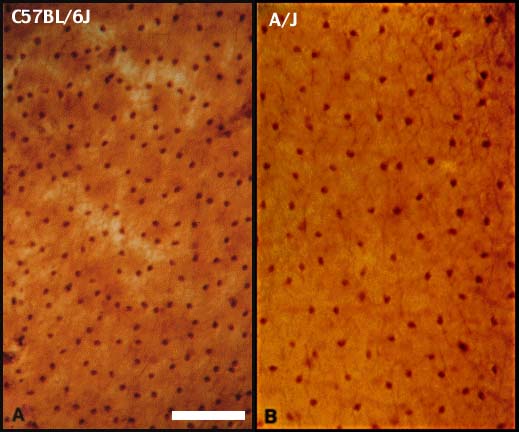
1998). Horizontal cells have a critical role in shaping the surround
responses of photoreceptors and bipolar cells (Sterling, 1998). We have
used an antibody directed against the 28 kDa calcium-binding molecule,
calbindin, to label essentially the entire population of horizontal
cells in the mouse (Figure 2).
There are very significant differences in densities of these cells
among the strains listed in Table 1. The greatest difference is between
C57BL/6J and A/J. As was true of retinal ganglion cells, heritability is
very high. We do not yet know how many genes influence the number and
density of calbindin-positive horizontal cells. However, the
intermediate density and the low variation within F1 hybrids from a
cross between A/J and C57BL/6J (see B6AF1/J in table 1) provides a
strong incentive to examine these cells in the set of 31 RI strains
generated by crossing A/J and C57BL/6J. It should be practical to map
major QTLs controlling variation in horizontal cell density and number.
From a functional perspective it is interesting to note that the ratio
of ganglion cells to horizontal cells varies from 3.2 to 6.7. Table 1. Two-fold variation in horizontal cell densities *Calbindin-positive horizontal cell density per 1 mm2.
The size of the eye is a important determinant of maximum light
gathering ability and of maximum acuity. Eye size is also a clinical
important trait because myopia—by far the most pervasive eye abnormality
in humans—is usually caused by excessive growth of the eye relative to
the refractive power of the cornea and lens. For these reasons we are
interested in determining whether there are QTLs that control the
overall growth of the eye. As above, the first step is to determine how
variable eye size is within and between strains of mice. Eye weight is
easy to measure and can be obtained rapidly for large numbers of
animals. Eye weight in the set of 11 strains listed in Table 2 varies
from 14.8 mg in SJL/J to 18.9 mg in CE/J. Three of the strains with
small eye weight are homozygous for the rd mutation in the beta
phosphodiesterase locus, and this association may be more than just
chance. Genetic factors in a broad sense account for approximately 30%
of the differences among cases. This is a high enough value to justify
an attempt to estimate numbers of genes affecting eye weight and then,
if possible, to locate and characterize underlying QTLs. Table 2. Eye weight, retinal area, and retinal ganglion cell
number * Three of these strains are homozygous rd mutants at the
phosphodiesterase locus. SE = Standard error of the mean, CV% is the coefficient of variation.
Eye weight is measured in mg. Retinal area is measured in mm2.
RGC is the population of retinal ganglion cells. Comparisons of weights
of unfixed right eyes and fixed left eyes reveal approximatelya 1 mg
weight loss (6%) following fixation. All of the eye weights listed below
are fixed weights. A regression analysis was used to neutralize a
significant age-related increase in eye weight. All weights are
normalized to 75 days. The correlation coefficient between eye weight
and retinal area is 0.75, that between weight and cell number is 0.44,
and that between area and number is 0.49. Numbers of QTLs affecting eye weight. If eye weight is
controlled by a large number of QTLs, then individual QTLs may not have
a large enough effect to be mapped. Our estimate of gene number is based
on a comparison of the variance in inbred strains and F1 and F2 progeny.
In contrast to ganglion cell number, a minimum of 10 QTLs appear to be
responsible for variation in eye weight. This estimate is two times
higher than a similar estimate generated by Lande (1981) using data from
Wilkens' classic genetic dissection of eye size in blind cavefish
(1971). If each of the 10 or more QTLs accounted for an equal fraction
of the genetic variance, then individual QTLs would have small effects
and would be hard to map. The 1.2 mg difference in Table 2 between C57BL/6J and DBA/2J is
interesting because these strains were used to generate the set of BXD
RI strains with which we succeeded in mapping the Nnc1 locus. To
map eye weight QTLs we compared the distribution of eye weights in BXD
strains with the distribution of alleles at more than 500 previously
mapped gene loci. A major QTL, Eye1, was mapped to proximal
chromosome 5 (Zhou and Williams, 1997, 1998).
This locus does not map near the beta phosphodiesterase locus or any of
the other 113 mutations that are known to affect eye and retinal
development in the mouse. To refine the position of Eye1 we are
now generating an advanced intercross (Darvasi, 1997) that should enable
us to map this locus to within 1–3 cM. We hope to be in a position to
test candidate genes that normally regulate growth of the eye over the
next few years. The analysis of genes controlling normal variation in vertebrates is
at an early stage. Our experience suggests that it will be practical to
map QTLs that have comparatively large phenotypic effects on most
heritable traits using RI strains and F2 intercrosses. As methods are
refined we should be able to map QTLs that have more subtle effects on
retinal and ocular traits. As increased numbers of QTLs are mapped, it
is likely that the same QTL will often be discovered repeatedly for
traits that were initially thought to be independent. Identifying QTLs
with pleiotropic effects has the potential of exposing common regulatory
and genetic mechanisms in different tissues. A good example is the
surprising common effects that cyclin D1 have on breast and retinal
development (Sicinski et al., 1995). Most developmental biologists are interested in understanding
molecular and cellular pathways that lead to the proliferation and
differentiation of cells and tissues. Their aim is to understood
representative organisms in ultimate detail. The molecular conservation
of metazoan development has resulted in a highly productive
cross-fertilization between research on nematodes, flies, fish, frogs,
birds, mice, and humans. But the appreciation of deep-rooted molecular
conservation has led to an unfortunate neglect of the genetic basis of
the remarkable variation within and among species. This variation is
primarily quantitative and is the untrampled research path that we have
chosen to explore. At one level of analysis, the QTLs that we are
isolating and characterizing are responsible for only minor variation in
retinal development. They do not produce dramatic mutations that garner
intense attention. But at another level of analysis, it is precisely
these variants that over many generations of selection have produced a
variety of eyes that are well adapted for vision in vastly different
environments. Acknowledgment. We thank Dr. Anand Swaroop for helpful
discussion. This work was supported by NEI RO1EY0662 to RWW. Research on
the Nnc1 locus is supported by NS35485 to RWW. Curcio CA, Sloan Jr. KA, Packer O, AE, Kalina RE (1987) Distribution
of cones in human and monkey retina: individual variability and radial
asymmetry. Science 236:576–582. Darvasi A (1997) Interval-specific congenic strains (ISCS): an
experimental design for mapping a QTL into a 1–centimorgan interval.
Mamm Gen 8:163–167. Hoskins SG (1985) Control of the development of the ipsilateral
retinothalamic projection in Xenopus laevis by thyroxine:
results and speculation. J Neurobiol 17:203–229. Lande R (1981) The minimum number of genes contributing to
quantitative variation between and within populations. Genetics
99:541–553. Lander ES, Botstein D (1989) Mapping Mendelian factors underlying
quantitative traits using RFLP linkage maps. Genetics 121:185–199. Lander ES, Schork NJ (1994) Genetic dissection of complex traits.
Science 265:2037–2048. Levinton J (1988) Genetics, paleontology, and macroevolution.
Cambridge UP, Cambridge. Nei M (1987) Molecular evolutionary genetics. Columbia UP, New
York. Rice DS, Williams RW, Goldowitz RW (1995) Genetic control of retinal
projections in inbred strains of albino mice. J Comp Neurol 354:459–469. Shoemaker DD, Lashkari DA, Morris D, Mittmann M, Davis RW (1996)
Quantitative phenotypic analysis of yeast deletion mutants using a
highly parallel molecular bar-coding strategy. Nat Gen 14:450–456. Sicinski P, Donaher JL, Parker SB, Li T, Fazelli A, Gardner H, Haslam
SZ, Bronson RT, Elledge SJ, Weinberg RA (1995) Cyclin D1 provides a link
between development and oncogenesis in the retina and breast. Cell
82:621–630. Sterling P (1998) Retina. In Synaptic organization of the brain,
4th Ed. (Shepherd GM, ed) Oxford UP, New York. Strom RC, Williams RW (1998) Developmental mechanisms responsible for
strain differences in the retinal ganglion cell populations.
J Neurosci 18:9948–9953 Tanksley SD (1993) Mapping polygenes. Annu Rev Genet 27:205–233. Walls GL (1942) The vertebrate eye and its adaptive radiation.
Cranbrook Inst Sci Bulletin 19, Bloomfield Hills, MI, USA. Wikler KC, Rakic P (1990) Distribution of photoreceptor subtypes in
the retina of diurnal and nocturnal primates. J Neurosci 10:3390–3401. Wikler KC, Williams RW, Rakic P (1990) Photoreceptor mosaic: number
and distribution of rods and cones in the rhesus monkey retina. J Comp
Neurol 297:499–508. Wilkens H (1971) Genetic interpretation of regressive evolutionary
processes: studies on hybrid eyes of two Astyanax cave
populations (Characideae, Pices). Evolution 25:530–544. Williams RW, Bastiani MJ, Lia B, Chalupa LM (1986) Growth cones,
dying axons, and developmental fluctuations in the fiber population of
the cat's optic nerve.
J Comp Neurol 246:32–69. Williams RW, Cavada C, Reinoso-Suárez F (1993) Rapid evolution of the
visual system: a cellular assay of the retina and dorsal lateral
geniculate nucleus of the Spanish wildcat and the domestic cat.
J Neurosci 13:208–228. Williams RW, Strom RC, Goldowitz D (1998) Natural variation in neuron
number in mice is linked to a major quantitative trait locus on Chr 11.
J Neurosci 18:138–146. Williams RW, Strom RC, Rice DS, Goldowitz D (1996) Genetic and
environmental control of variation in retinal ganglion cells number in
mice.
J Neurosci 16:7193–7205. Zhou G, Williams RW (1997) Mapping genes that control variation in
eye weight, retinal area, and retinal cell density. Soc Neurosci Abst
23:864. [see Invest Ophthalmol Vis Sci
40: 817–825.]
Since 11 August 98
|
||||||||||||||||||||||||||||||||||||||||||||||||||||||||||||||||||||||||||||||||||||||||||||||||||||||||||||||||||||||||||||||||||||||||||||||||||||||||||||||||
Neurogenetics at University of Tennessee Health Science Center
| Print Friendly | Top of Page |
Mouse Brain Library | Related Sites | Complextrait.org
